The Modern Computer
The modern
computer has become almost an appliance, to be used by a variety of people for
a
number of tasks. Admittedly, one of the
tasks is to be programmed and execute those programs;
in this it shares the heritage of the PDP–11/20 shown above. Your author’s first acquaintance
with computers was as equation solvers.
We had numerical problems to solve, and the easiest
way to do that was to use a computer.
The typical output was pages and pages of printed data;
the danger being that one would fall asleep from boredom before understanding
the results.
In addition to
serving as a number cruncher, the modern computer has many additional
tasks.
These illustrate the idea of a computer as a complete system with hardware as
only one part. As
an example of a modern computer, your author presents a picture and description
of the Acer
Netbook similar to that he bought for his wife in November 2010. The figure below was taken
from the Acer web site (http://us.acer.com/ac/en/US/content/group/netbooks).
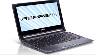
While not the
point of this chapter, we might as well give the technical specifications of
this
device. It is approximately 11 inches by
7.5 inches. When closed it is a bit less
than one inch
thick. This CPU model was introduced in
the second quarter of 2010. It is made
in China.
Here are more
specifications, using language that we will explain as a part of this course.
Some of the data below is taken from the stickers on the case of the
computer. Other
information is from the Intel web site [R001].
·
The
CPU is an Intel Core i3–330UM, which operates at 1.2 GHz.
It is described by Intel as “an Ultra Low Voltage dual–core processor
for small and light laptops.
·
It
has a three–level cache. Each of the two
cores has a L1 (Level 1) cache
(likely a 32–kilobyte split cache, with 16 KB for instructions and 16 KB for
data), and a 512 KB L2 cache. The two
cores share a common 3 MB L3 cache.
·
The
computer has 2 GB (2,048 MB) of DDR3 memory.
The maximum memory bandwidth is 12.8 GB/second.
·
The
computer has a 256 GB hard disk and two USB ports that can be used
for USB “flash” drives. The hard disk is
likely a SATA drive.
·
The
display is a 1366 by 768 “LED LCD”.
·
The
computer has a built–in GSM card for access to the global Internet
through the AT&T wireless telephone network.
The author
wishes to congratulate those readers who understood the above description
completely. A good part of this textbook
will be devoted to explaining those terms.
We now
turn to the main topic of this chapter.
How should we view a modern computer?
The best
description of this computer as an integrated system relates to the next
picture.
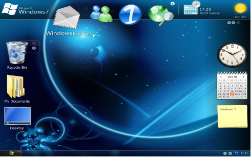
This figure
shows the GUI (Graphical User Interface) for a beta release of Windows 7. While
the final version of Windows 7 probably has a somewhat different appearance,
this figure is
better at illustrating the concept of a computer as an entire system.
The Virtual Machine Concept
Another way to
grasp this idea of the computer as a system comprising hardware, software,
networks, and the graphical user interface is to introduce the idea of a virtual machine. Those
students who have programmed in the Java programming language should have heard
of the
JVM (Java Virtual Machine). In this, we imagine that we have a computer
that directly
executes the Java byte code emitted by the Java compiler. While such a computer could be built,
and would then be a real machine, the most common approach is to run the JVM as
software on
an existing hardware platform. This idea
of virtual machines translates well into our discussion
here. What is the computer doing for
you? Is it an appliance for running a
web browser? If so,
you might have very little interest in the computer’s ISA (Instruction Set Architecture). If the
e–mail works and you can access Facebook, that might be all you are interested
in. OK, maybe
we need to add some MMOG (Massively Multiplayer Online Games) and Second Life to boot.
Anyone for “World of Warcraft” (worldofwarcraft.us.battle.net)?
Another way to
look at this “top level” of the computer is to consider the image above. One
might think of a computer as a device that does things when one clicks on
icons. It was not
always that way. Even after the video
display was first used, the menus were old DOS–style text
menus that were difficult to navigate.
As an example, your author recalls a NASA web site with
an interface that was text based. This
was rather difficult to use; in the end it was not worth the
trouble to find anything. It was
basically the same computer then as now (though today’s
version is a lot faster). What differs
is the software.
One view of
virtual machines focuses on the programming process. The basic idea is that there
is a machine to be programmed in a language appropriate to its logical
complexity. In the usage
suggested by Tanenbaum [R002], the lowest level of the computer, called “M0”, corresponds to
the digital logic in the Central Processing Unit. Its low level language, called “L0”, is hardly a
language at all. It is a description of
the digital signals that control the CPU and run through the
datapaths of the CPU to enable the computation.
This course will describe this low level an a bit
of detail. A complete study of this
level is more properly the subject of a course on Computer
Architecture, such as CPSC 5155 at Columbus State University.
The following
figure is adapted from Tanenbaum [R002], with addition of an additional level,
which your author calls “Level 6 – Application”. We now discuss a bit of this idea and relate
it
to the systems approach to considering computer organization.
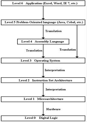 The idea of the
virtual machine concept is that
The idea of the
virtual machine concept is that
any computer is profitably studied as having a
number of levels. The true computer is
found at
Level 0; it is machine M0 with
language L0.
In this scheme,
the lowest level language, L0, is
easiest to process using standard digital gates. It
is also the most difficult for humans to understand.
The higher levels are easier for
humans, but more difficult for machines.
Upon
occasion, machines have been built that can
directly execute a Level 5 language in hardware,
but these are complex and far too rigid for any
commercial use.
Conceptually, we
have a sequence of machines,
each with its own language. In practical
terms,
we have a top to bottom flow, in which an
instruction in Level (N) is transformed into an
equivalent sequence of instructions at Level
(N – 1).
Note that Level
5 connects to both Level 4 and
Level 3, reflecting two options for a compiler.
Note that there
are two ways in which a sequence of instructions at one level can be
transformed
into a sequence of instructions at the next lower level. These are interpretation and
translation. In interpretation, software written in the
lower level language reads, interprets, and
carries out each instruction in turn.
The JVM (Java Virtual Machine) is a good example of
interpretation. There are two names
associated with translation: compilation
(when a Level 5
language is translated) and assembly
(when a Level 4 language is translated).
We should note
that there is some ambiguity in these terms.
We speak of Java source code being compiled into
Java byte code, which is then interpreted by the JVM. This is a possibly important distinction
that has very few practical effects on our discussions.
We note the two
options for translation of a Level 5 language.
On the IBM mainframes, these
languages are first converted to IBM Assembler Language and then assembled into
binary
machine language. This is similar to the
.NET architecture, in which a Level 5 language is first
converted into an intermediate language before being compiled to machine
language. We shall
return to the two–stage IBM process in just a bit.
While the flow
in the above diagram is obviously top to bottom, it is more easily explained in
a
bottom to top fashion, in which each virtual machine adds functionality to the
VM below it. As
noted above, the machine at level 0 is called “M0”. It comprises basic
digital gates activated by
control signals. It is these control
signals that make the computer work. At
this level, the focus
is on individual control signals, individual registers and memory devices, etc.
Machine M1 operates at the micro–instruction
level, translating these into control signals.
Consider a simple register addition. The
micro–instruction would connect the two source
registers to the adder, cause it to add, and connect the output to the
destination register. A
sample micro–instruction is as follows: R1 ®
B1, R2 ® B2, ADD, B3 ® R3. This is read as
one register loads bus B1 with its contents while another register loads B2,
the ALU (Arithmetic
Logic Unit) adds the contents of busses B1 and B2 and places the sum onto bus
B3, from whence
it is copied into the third register. At
this level, one might focus on the entire register file
(possibly 8, 16, or 32 general purpose registers), and the data path, over
which data flow.
Machine M2 operates at the binary machine
language level. Roughly speaking, a
binary
machine language statement is a direct 1–to–1 translation of an assembly
language statement.
This is the level that is described in documents such as the “IBM System/360
Principles of
Operation”. The language of this level
is L2, binary machine language.
Machine M3 has a language that is almost
identical to L2, the language of the level below it.
The main difference can be seen in the assembly output of an IBM COBOL
compiler. Along
with many assembly language instructions (and their translation into machine
language), one will
note a large number of calls to operating system utilities. As mentioned above, one of the main
functions of an operating system can be stated as creating a machine that is
easier to program.
We might mention the BIOS (Basic Input / Output System) on early Intel machines running
MS–DOS. These were routines, commonly
stored in ROM (Read Only Memory) that served to
make the I/O process seem more logical.
This shielded the programmer (assembly language or
higher level language) from the necessity of understanding the complexities of
the I/O hardware.
In the virtual
machine conceptualization, the operating system functions mainly to adapt the
primitive and simplistic low–level machine (the bare hardware) into a logical
machine that is
pleasing and easy to use. At the lowest
levels, the computer must be handled on its own terms;
the instructions are binary machine language and the data are represented in
binary form. All
input to the computer involves signals, called “interrupts”, and binary bits transferred either
serially or in parallel.
The study of
assembly language focuses on the ISA
(Instruction Set Architecture) of a
specific
computer. At this level, still rather
low level, the focus must be on writing instructions that are
adapted to the structure of the CPU itself.
In some ways, the Level 4 machine, M4,
is quite
similar to M2. At Level 4, however, one
finds many more calls to system routines and other
services provided by the Operating System.
What we have at this level is not just the bare CPU,
but a fully functional machine capable of providing memory management,
sophisticated I/O, etc.
As we move to
higher levels, the structure of the solution and all of the statements
associated
with that solution tend to focus more on the logic of the problem itself,
independent of the
platform on which the program executes.
Thus, one finds that most (if not all) Java programs
will run unmodified on any computing platform with a JVM. It is quite a chore to translate the
assembly language of one machine (say the IBM S/370) into equivalent language
to run on
another machine (say a Pentium).
The Level 5
machine, M5, can be considered to execute a high level language directly. In a
sense, the JVM is a Level 5 machine, though it does interpret byte code and not
source code.
At the highest
level of abstraction, the computer is not programmed at all. It is just used.
Consider again the screen shot above.
One just moves the mouse cursor and clicks a mouse
button in order to execute the program.
It may be working an Excel spreadsheet, connecting to
the World Wide Web, checking one’s e–mail, or any of a few thousand more
tasks. As has been
said before, at this level the computer has become an appliance.
What has enabled
the average user to interact with the computer as if it were a well–behaved
service animal, rather that the brute beast it really is? The answer again is well–written
software.
Occasionally, the low–level beast breaks through, as when the “blue screen of death” (officially
the “Stop Error” [R003]) is displayed when the computer crashes and must be manually
restarted. Fortunately, this is
happening less and less these days.
The Lessons from RISC
One of the
lessons from the RISC (Reduced Instruction Set Computer) movement again points
to
the idea that the computer is best seen as a hardware/software complete
system. The details of
the RISC designs are not important at this point; they will be mentioned later
in this course and
studied at some detail in any course on Computer Architecture, such as CPSC
5155 at Columbus
State University. The performance of any
computer depends on a well–crafted compiler well
matched to the Instruction Set Architecture of the Central Processing
Unit. One of the ideas
behind the RISC movement is that the hardware in the CPU be simpler, thus
leading to a simpler
machine language. The idea is that a
well–written compiler can translate a complex high–level
program into these simple machine language instructions for faster execution on
the simpler
hardware. Again, the compiler is
software. Even the process of software
execution should be
considered as a mix of software and hardware concerns.
The Computer as an Information Appliance
One aspect of
the use of a computer that is being seen more and more is that it is seen as an
information appliance. Specifically, the
user does not program the computer, but uses the
programs already loaded to access information, most commonly from the global
Internet. This
leads one to view the computer as a client node in a very large network of
information providers.
We shall discuss the client/server model
in some detail later. For now, we just
note that there
are some computers that are almost always connected to the global
Internet. These devices,
called servers, accept incoming messages, process them, and return information
as requested.
These are the server nodes. The client
nodes are intermittently connected to the global Internet,
when they request services from the server nodes. The period during which a client node is
linked to a server node is called a session.
Were it not for
the global Internet, the number of computers in general use would be only a
fraction of what it is today. Again, the
modern computer must be seen as a complete system.
As Dr. Rob Williams notes in his textbook [R004]
“It is clear that computers and
networks require both hardware and software in order
to work. … we will treat CSA [Computer
Systems Architecture] as a study if the
interaction of hardware and software which determines the performance of
networked computer systems.”
Dr. Williams
appears to be a fan of football, which we Americans call “soccer”. What follows
is a paraphrase of his analogy of the distinction between hardware and
software. As it is not
exactly a quotation, it is shown without quotation marks.
The distinction between hardware and software can be
likened between the distant
relationship between the formal photograph of a basketball team, rigidly posed
in front
of the basketball goal, and the exciting unpredictability of the NBA playoff
games.
The static photograph of the players only vaguely hints at the limitless possibilities
of
the dynamic game.
Developments in Hardware
As this is a
textbook on computer organization, we probably ought to say something about the
progress in hardware. The reader should
consult any one of a number of excellent textbooks on
Computer Organization and Architecture for a historical explanation of the
evolution of the
circuit elements used in computers. The
modern computer age can be said to have started with
the introduction of the IC (Integrated Circuit) in the early 1970’s.
Prior to
integrated circuits, computers were built from discrete parts that were
connected by
wires. The integrated circuit allowed
for the components and the wires connecting them to be
placed on a single silicon die (the plural of “die” is “dice”; think of the
game). The perfection of
automated fabrication technologies lead to the development of integrated
circuits of ever more
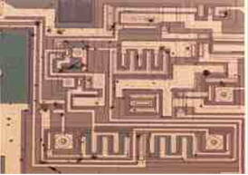
increasing complexity. The next figure
shows an early integrated circuit. What
appears to be
long straight lines are in fact traces,
which are strips of conductive material placed on the chip to
serve as wires conducting electrical signals.
Some of the larger components are likely transistors
directly fabricated on the chip.
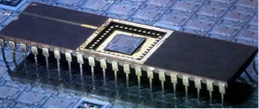
The early
integrated circuit chips were housed in a larger structure in order to allow
them to be
connected on a circuit board. Here is a
picture of a DIP (Dual In–line Pin) chip.
This chip
appears to have forty pins, twenty on this side and twenty on the opposite
side.
One of the main
advantages of integrated circuits is seen by comparison with the backplane of a
computer from 1961. This is the Z23,
developed by Konrad Zuse.
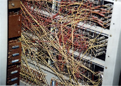 What the reader
should notice here is the entangled sets
What the reader
should notice here is the entangled sets
of wires that are connecting the components.
It is
precisely this wiring problem that gave rise to the
original integrated circuits. If the
components of a circuit
and the connecting wires could be etched onto a silicon
surface, the complexity of the interconnections would be
greatly decreased. This would yield an
improvement in
the quality control and a decrease in the cost of
manufacture.
It should be no news to anyone that
electronic computers have progressed impressively in
power since they were first introduced about 1950. One of the causes of this progress has
been the constant innovation in technology with which to implement the digital
circuits.
The last phase of this progress, beginning about 1972, was the introduction of
single–chip
CPUs. These were first fabricated with LSI (Large Scale Integrated) circuit technology, and
then with VLSI (Very Large Scale Integrated) circuitry. As we trace the later development
of CPUs, beginning about 1988, we see a phenomenal increase in the number of
transistors
placed on CPU chip, without a corresponding increase in chip area.
There
are a number of factors contributing to the increased computing power of modern
CPU chips. All are directly or
indirectly due to the increased transistor density found on
those chips. Remember that the CPU
contains a number of standard circuit elements, each
of which has a fixed number of transistors.
Thus, an increase in the number of transistors on
a chip directly translates to an increase in either the number of logic
circuits on the chip, or
the amount of cache memory on a chip, or both.
Specific benefits of this increase include:
1. Decreased
transmission path lengths, allowing an increase in clock frequency.
2. The
possibility of incorporating more advanced execution units on the CPU. For
example, a pipelined CPU is
much faster, but requires considerable circuitry.
3. The
use of on–chip caches, which are considerably faster than either off–chip
caches or primary DRAM.
For VLSI
implementations of CPU chips, the increase in transistor count has followed
what
is commonly called “Moore’s Law”. Named
for Gordon Moore, the co–founder of Intel
Corporation, this is an observation on the number of transistors found on a
fixed–sized
integrated circuit. While not
technically in the form of a law, the statement is so named
because the terms “Moore’s Observation”, “Moore’s Conjecture” and “Moore’s
Lucky
Guess” lack the pizazz that we expect for the names of popular statements.
In a previous
chapter, we have shown a graph of transistor count vs. year that represents one
statement of Moore’s Law. Here is a more
recent graph from a 2009 paper [R005].
The
vertical axis (logarithmic scale) represents the transistor count on a typical
VLSI circuit.
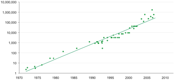
By itself,
Moore’s law has little direct implication for the complexity of CPU chips. What it
really says is that this transistor count is available, if one wants to use
it. Indeed, one does
want to use it. There are many design
strategies, such as variations of CPU pipelining
(discussed later in this textbook), that require a significant increase in
transistor count on the
CPU chip. These design strategies yield
significant improvements in CPU performance, and
Moore’s law indicates that the transistor counts can be increased to satisfy
those strategies.
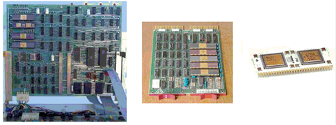
We see an
earlier result of Moore’s Law in the next figure, which compares Central
Processing
Units from three implementations of the PDP–11 architecture in the 1980’s. Each circuit
implements the same functionality. The
chip at the right is about the same size as one of the five
chips seen in the right part of the central figure.
The utility of Moore’s Law for our discussion is the
fact that the hardware development that it
predicted has given rise to very impressive computing power that we as software
developers
have the opportunity to use. One of the
more obvious examples of this opportunity is the recent
emergence of GPUs (Graphical Processing Units), which
yield high–quality graphics at
reasonable costs, leading to the emergence of the video game industry.
The Power Wall
While the
increase in computing power of CPUs was predicted by Moore’s Law and occurred
as
expected, there was an unexpected side–effect that caught the industry by
surprise. This effect
has been given the name “The Power Wall”.
Central Processing Units became more powerful
primarily due to an increase in clock speed and an increase in circuit
complexity, which allowed
for more sophisticated logic that could process instructions more quickly.
What happened is
that the power consumed by the CPU began to grow quickly as the designs
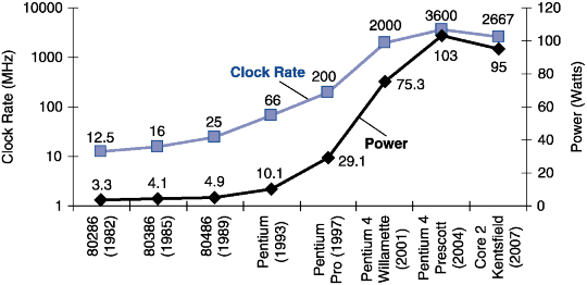
incorporated faster clocks and more execution circuitry. In the next figure we see the clock
speeds and power consumptions of a number of CPUs in the Intel product
line. The high point
in both clock speed and power consumption was the Prescott in 2004. The following figure
was taken from the textbook by Patterson and Hennessy [R007].
So far, so good;
the power supplies have never been an issue in computer design. However, all
the power input to a CPU chip as electricity must be released as heat. This is a fundamental law
of physics. The real problem is the
areal power density; power in watts divided by surface area
in square centimeters. More power per
square centimeter means that the temperature of the
surface area (and hence the interior) of the CPU becomes excessive.
The Prescott was
an early model in the architecture that Intel called “NetBurst”,
which was
intended to be scaled up eventually to ten
gigahertz. The heat problems could
never be
handled, and Intel abandoned the architecture.
The Prescott idled at 50 degrees Celsius (122
degrees Fahrenheit). Even equipped with
the massive Akasa King Copper heat sink , the
system reached 77 Celsius (171 F) when operating at 3.8 GHz under full load and
shut itself
down.
As noted above,
increasing the power to a CPU without increasing its area must lead to an
increase in the power density and hence the operating temperature of the
CPU. Unfortunately,
this increased the power dissipation of the CPU chip beyond the capacity of
inexpensive cooling
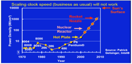
techniques. Here is a slide from a talk
by Katherine Yelick of Lawrence Berkeley National Lab
[R006] that shows the increase of power density (watts per square centimeter)
resulting from the
increase in clock speed of modern CPUs. The
power density of a P6 approaches that of a shirt
iron operating on the “cotton” setting. One
does not want to use a CPU to iron a shirt.
Later in the
text we shall examine some of the changes in CPU design that have resulted from
problem of heat dissipation.
Overview of CPU Organization
The modern computer is a part of a classification called
either a von Neumann machine or a
stored
program computer.
The two terms are synonyms. The
idea is that the computer is a
general purpose machine that
executes a program that has been read into its memory. There are
special purpose computers, which
execute a fixed program only. While
these are commercially
quite significant, we shall not
mention them to any great extent in this course.
Stored program computers have four major components: the CPU
(Central Processing Unit), the
memory, I/O devices, and one or more
bus structures to allow the other three components to
communicate. The figure below illustrates the logical organization.
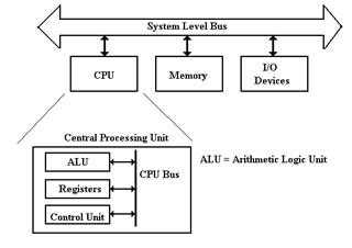
Figure: Top-Level Structure of a Computer
The functions of the three top-level components of a
computer seem to be obvious. The I/O
devices allow for communication of
data to other devices and the users. The
memory stores both
executable code in the form of
binary machine language and data. The CPU
comprises
components that execute the machine
language of the computer. Within the
CPU, it is the
function of the control unit to interpret the machine language and cause the CPU to
execute the
instructions as written. The Arithmetic
Logic Unit (ALU) is that component of the CPU that
does the arithmetic operations and
the logical comparisons that are necessary for program
execution. The ALU uses a number of local storage units,
called registers, to hold results of
its operations. The set of registers is sometimes called the register file.
Fetch-Execute Cycle
As we shall see, the fetch-execute
cycle forms the basis for operation of a stored-program
computer. The CPU fetches each instruction from the
memory unit, then executes that
instruction, and fetches the next
instruction. An exception to the “fetch
next instruction” rule
comes when the equivalent of a Jump
or Go To instruction is executed, in which case the
instruction at the indicated address
is fetched and executed.
Registers vs. Memory
Registers and memory are similar in that both store
data. The difference between the two is
somewhat an artifact of the history
of computation, which has become solidified in all current
architectures. The basic difference between devices used as
registers and devices used for
memory storage is that registers are
usually faster and more expensive (see below for a
discussion of registers and Level–1
Cache).
The origin of the register vs. memory distinction can be
traced to two computers, each of which
was built in the 1940’s: the ENIAC (Electronic Numerical Integrator and Calculator – becoming
operational in 1945) and the EDSAC (Electronic Delay Storage Automatic Calculator –
becoming operational in 1949). Each of the two computers could have been
built with registers
and memory implemented with vacuum
tubes – a technology current and well-understood in the
1940’s. The difficulty is that such a design would
require a very large number of vacuum tubes,
with the associated cost and
reliability problems. The ENIAC solution
was to use vacuum tubes
in design of the registers (each of
which required 550 vacuum tubes) and not to have a memory
at all. The EDSAC solution was to use vacuum tubes in
the design of the registers and mercury
delay lines for the memory unit.
In modern computers, the CPU is usually implemented on a
single chip. Within this context, the
difference between registers and
memory is that the registers are on the CPU chip while most
memory is on a different chip. Now that L1 (level 1) caches are appearing on
CPU chips (all
Pentium™ computers have a 32 KB L1
cache), the main difference between the two is the
method used by the assembly language
to access each. Memory is accessed by
address as if it
were in the main memory that is not
on the chip and the memory management unit will map the
access to the cache memory as
appropriate. Register memory is accessed
directly by specific
instructions. One of the current issues in computer design
is dividing the CPU chip space
between registers and L1 cache: do
we have more registers or more L1 cache?
The current
answer is that it does not seem to
make a difference.
The C/C++ Programming Language
A good part of
the course for which this text is written will concern itself with the internal
representations of data and instructions in a computer when running a
program. Items of interest
include the hexadecimal representations of the following: the machine language
instructions, the
values in the registers, the values in various memory locations, the addressing
mechanisms used
to associate variables with memory locations, and the status of the call
stack. The best way to do
this is to run a program and look at these values using a debugger that shows
hexadecimal
values. Following the lead of Dr. Rob
Williams, your author has chosen to use the Microsoft
Visual Studio 8 development environment, and use the language that might be
called “C/C++”.
The C programming
language was developed between 1969 and 1973 by Dennis Ritchie at the
Bell Laboratories for use with the Unix operating system. This is a very powerful programming
language, which is full of surprises for the inexperienced programmer. The C++ language was
developed by Bjarne Stroustrup, also of Bell laboratories, beginning in
1979. It was envisioned
as an improved version of the C language, and originally called “C with
Classes”. It was
renamed C++ in 1983.
Your author’s
non–standard name “C/C++” reflects the use we shall make of the programs
written as examples. For the most part
the program will be standard C code, compiled by a
C++ compiler. For this course, it is
sufficient to have “C++ without classes”.
The major
difference between our C/C++ and the standard C language is that the old printf
routine is not used, being replaced by the C++ cout (say “See–out”) output stream. This
is seen in comparing two versions of the standard Hello World program.
Here is the
program, as written in standard C.
#include <stdio.h>
main( ) {
printf("Hello,
world! \n");
return 0;
}
Here is the program, as written in
standard C++.
#include <iostream>
using namespace std; // Allows
standard operators to be used.
main( ) {
cout << "Hello,
world!” << endl;
return 0;
}
Another notable
difference is found in the handling of subprograms. In Java, it is common to
call these “methods”, whether or not
they return a value. In both C and C++,
these are called
“functions”. What some would call a
subroutine, each of these languages calls a “function
returning void”.
Another issue of
interest is the syntax for declaring and calling functions with arguments
called
by reference. The standard example of
this is the swap or flip function, which
swaps the
values of its arguments. We shall
discuss a function to swap the values of integer variables.
The C approach
is dictated by the fact that all arguments are passed by value. The value to
be passed here is not that of the variable but its address. The value of the address can then be
used to reference and change the value of the variable.
flip(int *x, int *y) // Pointers
{
int temp;
temp = *x;
// Get value pointed to by *x
*x = *y;
*y = temp;
}
This function is
called as follows.
flip (&a, &b); // Passes pointers to a and b
The C++ approach is somewhat
different. Here is the function again,
seen within a complete
program. The screen shot shows the
compiled C++ code that your author was able to run. Line
23 shows an apparently useless input operation; the input value is never used. The reason for
this is to freeze the output screen so that it can be viewed. Lines 4 and 15 were created
automatically by the IDE.
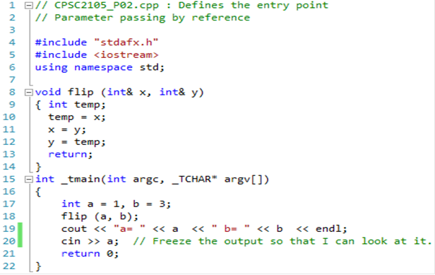
The standard C
code at the top of this page is shown just for comment. The C++ code, seen in
the screen shot, is more typical of the types of programs that will be required
for the course for
which this text was written. The focus
will be on running small programs and using the
debugger to observe the internal structures.
Setting Up for Debugging
The appendix, MS Visual Studio 8, Express Edition,
in the book by Dr. Rob Williams has
some valuable suggestions for configuring the IDE to give valuable debug
information. Here
are some more hints. All that your
author can claim here is that these worked for him.
1. Create the project and enter the source
code, saving everything as appropriate.
2. Right mouse click on the menu bar just
below the close [X] button.
Select the Debug, Standard, and
Text Edit windows.
3. Go to the Debug menu item and select
“Options and Settings”.
Go to the General options and
check the box “Enable address–level debugging”
4 Go to the Tools menu item and select
“Customize”. Select the Debug toolbar
and anything else you want.
5. Place the mouse cursor on the left of one
of the line numbers in the code listing.
Left click to highlight the line.
6. Go to the Debug menu item and click
“Toggle Breakpoint”.
Function key [F9] will do the
same thing.
7. Start the debugger. Wait for the program to build and begin
execution.
8. After the program has stopped at the
breakpoint, go to the Debug menu item,
select “Windows” and select the
following window (some will be already selected):
Breakpoints, Output, Autos,
Locals, Call Stack, Memory, Disassembly, and Registers.
9. Select a tab from the bottom left window
and view the contents. Your author’s IDE
shows
these tabs: Autos, Locals, Memory
1, Memory 2, Registers, Threads, and a few more.
10. Notice the command prompt on the bottom bar
of Windows. Click on this
to see where the output will go.
References
[R001]
http://ark.intel.com/products/49021/Intel-Core-i3-330UM-Processor-(3M-cache-1_20-GHz)
This web site accessed July 16, 2011
[R002] Andrew S. Tanenbaum, Structured Computer Organization, Pearson/Prentice–Hall,
Fifth Edition, 2006, ISBN 0
– 13 – 148521 – 0.
[R003] http://en.wikipedia.org/wiki/Blue_Screen_of_Death,
accessed July 18, 2011
[R004] Rob Williams, Computer Systems Architecture:
A Networking Approach,
Pearson/Prentice–Hall,
Second Edition, 2006, ISBN 0 – 32 – 134079 – 5.
[R005] Jonathan G. Koomey,
Stephen Berard, Marla Sanchez, & Henry Wong;
Assessing Trends in the Electrical Efficiency of Computation Over Time,
Final Report to Microsoft
Corporation and Intel Corporation, submitted to
the IEEE Annals of the History
of Computing on August 5, 2009.
[R006] Katherine Yelick,
Multicore: Fallout of a Hardware
Revolution.
[R007] David A. Patterson & John L. Hennessy, Computer Organization and Design:
The Hardware/Software
Interface, Morgan Kaufmann, 2005,
ISBN 1 – 55860 – 604 – 1.
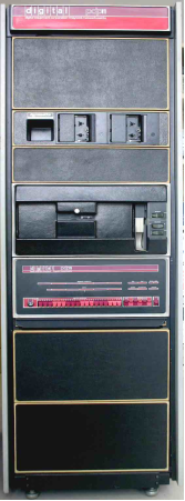 The PDP–11 was a
16–bit processor introduced by the Digital
The PDP–11 was a
16–bit processor introduced by the Digital