Subprograms: Subroutines, Procedures, and Functions

The Context of the Subprogram Call

As the last executable statement, a subprogram must return to the address just following the
instruction that invoked it. It does this by executing a branch or unconditional jump to an
address that has been stored appropriately.

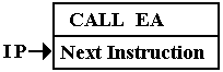
Here is a bit more on the context of a subroutine call instruction. Let EA denote the Effective
Address of the subprogram to be called. The situation just before the call is shown below. At
this point, the IP (Instruction Pointer) had already been moved to the next instruction.

The execution of the CALL involves three tasks:

1. Computing the value of the Effective Address (EA).

2. Storing the current value of the Instruction Pointer (IP)
so that it can be retrieved when the subroutine returns.

3. Setting the IP = EA, the address of the first instruction in the subroutine.

Here we should note that this mechanism is general; it is used for all subroutine linkage
protocols. What differs is the handling of the return address.

Storing the Return Address

The simplest method for storing the return address is to store it in the subroutine itself. This
mechanism allocates the first word of the subroutine to store the return address. The next
figure shows how this was done in the CDC–6600, an early supercomputer with word
addressing, so that the instruction following address Z is at address (Z + 1).

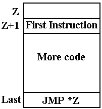
If the subroutine is at address Z in a word–addressable machine such as the Boz–5, then

Address Z holds the return address.

Address (Z + 1) holds the first executable instruction of the subroutine.

JMP *Z An indirect jump on Z is the last instruction of the subroutine.
Since Z holds the return address, this affects the return.

This is a very efficient mechanism. The difficulty is that it cannot support recursion.

An Aside: Static and Dynamic Memory Allocation

The efficiency of the early memory allocation strategies was also a source of some rigidity. All
programs and data were loaded at fixed memory locations when the executable was built. Later
modifications allowed the operating system to relocate code as required, but the essential model
was fixed memory locations for each item.

Most early modifications of the static memory allocation strategy focused on facilitation of the
program loader. One mechanism, undertaken in 1960 by IBM for a variety of reasons, was to
make almost all memory addresses relative to the start address of the program. The mechanism
was built on the use of a base register, which was initialized to the program start address. When
the operating system relocated the code to a new address, the only change was the value of that
base address. This solved many problems, but could not support modern programming styles.

Modern computer programming style calls for use of recursion in many important cases. The
factorial function is one of the standard examples of recursion. The code serves as a definition
of the factorial function. The only non–standard modification seen in this code is that it returns
the value 1 for any input less than 2. The mere fact that the factorial of –1 is not defined should
be no excuse for crashing the code. Does the reader have a better idea?

   Integer Factorial (Integer N)
     If (N < 2) Then Return 1 ;
                Else Return N*Factorial(N – 1);

Dynamic memory allocation was devised in order to support recursive programming and also a
number of other desirable features, such as linked lists and trees. The modern design calls for an
area of memory that can be allocated to dynamic allocation. The two important structures in this
area are the stack and the heap. The stack is used to store the return address for a subprogram,
the arguments to that subprogram, and the variables local to that program. The heap is used to
store dynamic data structures, created by the new operator in Java or malloc() in C and C++.

Actual physical memory on a computer is a fixed asset, so the designers had to decide how much
to allocate to the stack and how much to allocate to the heap. An obvious simplification was
quickly agreed upon; they would specify the total amount of memory allocated to both. The
stack would be allocated from high memory and grow towards low memory. The heap would
be allocated from low memory and grow towards high memory. As long as the two did not
overlap, the available memory could be shared without the artificiality of a partition.

Here is as memory map showing the allocation for a computer in the MIPS–32 line. This is a
modern microprocessor, commonly used in embedded applications.

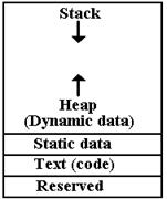The stack begins at 32–bit address 0x7FFF FFC and grows toward
smaller values. The static data begins at address 0x1000 8000
and occupies an area above that address that is fixed in size when
the program is loaded into memory.

The dynamic data area is allocated above the static data area and
grows toward higher addresses.

Note that some data are allocated statically to fixed memory addresses
even in this design. In C and C++, these would be variables declared
outside of functions, retaining value for the life of the program.

The IA–32 Implementation of the Stack

It is important to make one point immediately. The discussion in this chapter will focus on the
IA–32 implementation of the stack and the protocols for subprogram invocation. However, the
mechanisms to be discussed are in general use for all modern computer architectures. The
register names may be different, but the overall strategy is the same.

There are a number of possible implementations of the ADT (Abstract Data Type) stack. This
text will focus on that implementation as used in the Intel IA–32 architecture, seen in the Intel
80386, Intel 80486, and most Pentium implementations. We have already shown why it was
decided to have the stack grow towards lower addresses; a PUSH operator decrements the
address stored in the stack pointer. We now explain the precise use of the stack pointer. There
are two possible models: the stack pointer indicates the address of the last item placed on the
stack, or the stack pointer indicates the location into which to place the next item. Both are valid
models, but only one can be used.

In the IA–32 architecture, the stack pointer is called ESP (Extended Stack Pointer). It is a
32–bit extension of the earlier 16–bit stack pointer, called SP. In this architecture, only
32–bit values are placed on the stack. As the IA–32 architecture calls for byte addressability and
each stack entry holds four bytes, the stack addresses differ by 4.

Here is a pseudo–code representation of the implementation of the two main stack operators.
While it may seem counterintuitive, the design calls for decrementing the ESP on a push to the
stack and incrementing it on a pop from the stack.

PUSH ESP = ESP - 4 // Decrement the stack pointer
MEM[ESP] = VALUE // Place the item on the stack

POP VALUE = MEM[ESP] // Get the value
ESP = ESP + 4 // Increment the stack pointer

At some time during the operating system load, the stack pointer, ESP, is given an initial address.
In the MIPS–32 design, the initial value is set at hexadecimal 0x7FFF FFFC. The 32–bit entry
at that address comprises bytes at addresses 0x7FFF FFFC, 0x7FFF FFFD, 0x7FFF FFFE,
and 0x7FFF FFFF. The next higher 32–bit address would be 0x8000 0000.

As a simpler illustration, consider the stack as might be implemented in a program running on
an IA–32 system. We imagine that the stack pointer (ESP) contains the address 0x00001000,
abbreviated in the figure to 0x1000. We begin with the stack containing one value. While all
items on the stack will be 32–bit values (eight hexadecimal digits), we use 4 digits to illustrate.

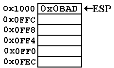At this point, ESP = 0x00001000, better represented as
0x0000 1000 to facilitate reading the value. The
figure shows this as 0x1000 to save space.

The decimal value 2,989 (hexadecimal 0x0BAD) is
stored at this address. The clever name is used to
indicate that a program can assume as good data only
what it actually places on the stack.

This discussion is adapted from Kip R. Irvine [R019].

The value 0x00A5 is pushed onto the stack.

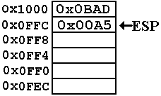
The address in the stack pointer is now
ESP = 0x0FFC.

In hexadecimal arithmetic 0x1000 – 4 = 0xFFC.

Value 0x0C represents decimal 12 and
value 0x10 represents decimal 16.

The value 0x0001 is pushed onto the stack.

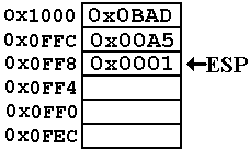
The address in the stack pointer is now
ESP = 0x0FF8.

Note that 0x08 + 0x04 = 0x0C, another way
of saying that 8 + 4 = 12 (decimal arithmetic).

A value is popped from the stack and placed in the 32–bit register EAX.

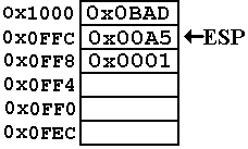Now we have the following values
ESP = 0x0FFC
EAX = 0x0001

Note that the value 0x0001 is not actually removed from
memory. Logically, it is no longer part of the stack. There
may be some security advantages to zeroing out a location
from which a value has been popped. I just don’t know.

The value 0x0002 is pushed onto the stack.

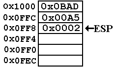Now again, ESP = 0x0FF8.

Note that the value in that address has been
overwritten. This is the standard implementation
of a stack. When a value is popped from the stack,
its memory location is no longer logically a part of the
stack, and is available for reuse.

Having given an introduction to the stack as implemented by the IA–32 architecture, we
consider the use that was first mentioned. The stack is used to store the return addresses.

Using a Stack for the Return Address

While a proper implementation of recursion depends on using the stack for more than just the
return addresses, we shall focus on that for the moment. Consider the following code fragment,
written in an entirely odd style with pseudo–code that uses labeled statements.

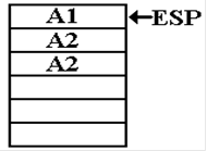
We begin with the code in the calling routine.

     N = 3
     M = FACT(N)
A1: J = M*3      // A silly statement, just to get the label

Here is a strange version of the called function, again with labels. The strange style, such as
use of three lines in order to write what might have been written as K1 = L*FACT(L – 1) is
due to the fact that the executing code is basically a collection of very simple assembly language
statements. There is also the fact that this illustration requires an explicit return address.

     INTEGER FACT (INTEGER L)
     K1 = 1 ;
     IF (L > 1) THEN
        L2 = L – 1;
        K2 = FACT(L2);
A2:     K1 = L*K2 ;
     END IF ;
     RETURN K1 ;

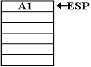
Here is the “story of the stack” when the code is called. When FACT is first called, with N = 3,
the return address A1 is placed onto the stack.

Again, we should note that the real implementation of this
recursive call requires the use of the stack for more than
just the return address.

This first illustration focuses on the return address and
ignores everything else.

The complete use of the stack will be the subject of much
of the rest of this chapter.

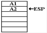
Here, the argument is L = 3, so the factorial function is called recursively with L = 2. The
return address within the function itself is pushed onto the stack.

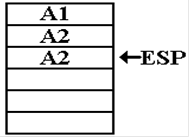
Now the argument is L = 2, so the function is called recursively with L = 1. Again, the
return address within the function is pushed onto the stack.

Now the argument is L = 1. The function returns with value 1. The address to which execution
returns is the address A2 within the function itself. Overlooking the very inconvenient difficulty
with establishing the value of the argument, we note the condition of the stack at that point.

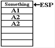
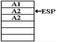Note that the second occurrence of the address A2 remains in
the memory location recently indicated by the stack pointer,
though it is no longer logically a part of the stack.

The computation continues, and the function produces the value 2. The next return is to the
address A2, which is popped from the stack. The stack condition is now as follows.

The function produces the value 6, by a method not indicated
in this discussion, and executes another return.

This time the return address is A1, the next line of code in the
procedure that called this function.

After the return, the state of the stack is as follows.

More Problems with Static Allocation

We have solved the problem of the management of return addresses for recursive subprograms
by introducing the dynamic data structure called the stack. What we are left with at this point
of our logical development is static allocation for the argument and local variables. As we shall
make abundantly clear, this will not work for recursive subprograms.

Consider the factorial function, as written in its strange form above, but with a few additional
lines that might also appear strange. Note the explicit static allocation of memory to hold four
local integer variables. In a higher level language, the compiler handles this automatically.

     INTEGER FACT (INTEGER L)
     K1 = 1 ;
     L1 = L ;
A3: IF (L1 > 1) THEN
        L2 = L1 – 1;
        K2 = FACT(L2);
A2:     K1 = L1*K2 ;
     END IF ;
     RETURN K1 ;
K1: DS INTEGER    // Set aside four bytes to store an integer
K2: DS INTEGER    // These four lines statically allocate
L1: DS INTEGER    // 16 bytes to store four integers.
L2: DS INTEGER

It might be interesting to note the evolution of values for all four variables, but it is necessary
only to look at two: K1 and L1. We watch the evolution at the conditional statement, newly
labeled A3. The label L1 is used to force our attention to the storage of the argument L.

When called with L = 3, the values are K1 = 1 and L1 = 3. FACT(2) is invoked.

When called with L = 2, the values are K1 = 1 and L1 = 2. FACT(1) is invoked.

When called with L = 1, the values are K1 = 1 and L1 = 1. The value 1 is returned.

But note what the static allocation of data has done to this recursive scheme. When the
function returns from K2 = FACT(L2), L1 ought to have the value 2. It does not, as
the proper value has been overwritten. There are two options for the function if implemented
in this style: either it returns a value of 1 for all arguments, or it crashes the computer.

Automatic Variables

As the problem with local variables in recursive subprograms arose from static allocation of
memory, any proper design must allow for allocation that is not static. Because a uniform
approach is always preferable to the creation of special cases, language designers have opted
to apply this allocation scheme to all subprograms, including those that are not recursive.

In general, variables are now divided into two classes: static and local. In the C and C++
languages, local variables are often called “automatic variables” as the memory for these is
automatically allocated by the compiler and run–time system.

In C and C++, static variables are considered to be those that are declared outside any
subprogram. In Java, these variables can be explicitly declared within a method. Those
variables explicitly declared as static retain their values between invocations of the method.
There are some valid uses for static variables, but they cannot be used for recursion.

If local variables are to be allocated automatically, what is to be the mechanism for doing so?
The answer has been to use the stack. The fact that the stack is also used to store return
addresses does have some implications for computer security. Despite that downside, the
mechanism is so convenient that it has been widely adopted.

There are two classes of data that are candidates for storage on the stack. The above illustration
of static allocation treated them together in order to make a point. We now differentiate the two.
There are arguments to be passed to the subprogram and variables local to that subprogram.

The protocol for passing arguments is easily described: push the arguments on the stack and
then, as a part of the CALL instruction, push the return address onto the stack. If the arguments
to the subprogram are pushed on the stack, then what is the order in which they are pushed?

There are two conventions, called the “Pascal Convention” and “C Convention”. In the
Pascal convention, used by the Pascal programming language, the arguments are pushed left to
right. In the C convention, the arguments are pushed right to left. Consider the following
subprogram invocation, in which L, M, and N are simple integer value parameters.

PROCA (L, M, N)

The sequence for a Pascal–like language would be
      PUSH L
      PUSH M
      PUSH N
      CALL PROCA

The sequence for a C–like language would be
      PUSH N
      PUSH M
      PUSH L
      CALL PROCA

For arguments that are passed by reference, the address of the argument is put onto the stack.
Consider the following line of C++ code, adapted from the book by Rob Williams.

n = average (10, math_scores)

This might be implemented in assembly language as follows:

      LEA EAX, math_scores // Get the address of the array
      PUSH EAX               // Push the address
      PUSH 0Ah               // Push hexadecimal A, decimal 10
      CALL average

What we have is an address pushed onto the stack, followed by a value. The CALL instruction
pushes the return address. As in many conventions, there is no abstract logical reason for
preferring one stack ordering over the other; we just must be consistent.

Again in our development of the protocol for subprogram linkage, we shall overlook a very
significant point, which will be introduced and justified later. At this point in the discussion,
the subprogram has been called and the stack populated appropriately. This text will assume the
calling conventions used in C and C++, so the state of the stack is as follows. After the call to
PROCA (L, M, N), the stack condition is as follows. RA denotes the return address.

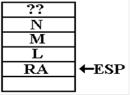The “??” at the top of this drawing is used to illustrate one
important feature of stack usage. Before the call to PROCA
something has been placed on the stack. However, the code
in PROCA must use only what was placed on the stack either
by the call to PROCA or by PROCA itself. Whatever else is
on the stack should be considered as unknowable. This basic
assumption allows the coder to treat PROCA as independent.

How is PROCA to gain access to the values on the stack? One way would be to POP the values
and place them in static storage within the procedure itself. There are two obvious objections to
this in addition to the fact that the first value popped from the stack would be the return address.

It is possible to handle the return address problem by reordering the use of the stack in the calling
procedure. While possible to push the return address first, such a choice leads to complication in
implementation of the subprogram call instruction. It is much easier to design a mechanism that
requires the return address to be pushed onto the stack just before subprogram invocation.

Another major problem with the above idea is that it returns to static allocation of memory, just
using the stack to transfer data from one procedure to another. The second objection to this
scheme had more importance in early computer designs: every argument is stored twice or
three times. Copying of values from the calling program to the stack may be necessary, but
copying of the values from the stack to the called subprogram is just wasteful.

The Stack as a NOT–ADT

At this point, we observe that the stack pointer, ESP, is just an address. The arguments to the
subprogram can be addressed relative to that address. At this point, before the subprogram has
done anything, argument L is at address (ESP + 4), argument M is at address (ESP + 8), etc.

We must make a few comments on these observations. First, we are assuming the usage that is
preferred for the Pentium and all other 32–bit designs. Only 32–bit (four byte) entries are placed
on the stack. We are also looking at the stack before the subprogram has done anything at all.
This condition will be discussed more fully once we have introduced the frame pointer.

The more significant point to be made is that we have given up on treating the run–time stack as
an ADT (Abstract Data Type). A stack, in the sense of a course in Data Structures, is an ADT
accessed only with a few basic operations such as PUSH, POP, IsEmpty, and possibly TOP. In
the ADT sense, the stack pointer is not visible to code outside that used to implement the stack.
At this point, and especially in what just follows in this discussion, the stack pointer is not only
visible to the code, but also is explicitly manipulated by that code.

The Final Touches on the Protocol

We are now at the stage where we can justify the protocol actually used in the Pentium, as
well as many other modern computers. Remember that the computer is to be seen as a true
combination of both hardware and software. The hardware can provide the registers to support
subprogram invocation, but there must be protocols for using that hardware. At the present time,
the IA–32 architecture (as used in many Pentium implementations) is best seen as both hardware
and protocols for writing the software.

Suppose that the procedure PROCA has a line of the form K = L + M + N. Setting aside the
very important issue of how to allocate memory for the local variable K, we might imagine
the use of addresses [ESP + 4], [ESP + 8], and [ESP + 12] (decimal numbering) to access the
values represented by the variables. But such a strategy makes a significant assumption that is
totally unwarranted; specifically it assumes that the stack pointer has not been altered by any
code between entry to the subroutine and the use of the arguments. (Again, please ignore the
fact that we know it has been so altered.)

If the stack is to be allowed to grow as the needs of the code require, we must assume that the
value in ESP will also change unpredictably. If the address stored in the stack pointer is to be
used reliably for access to the arguments, the only solution is to copy it to another location. The
choice made by most designers is to use another register, often called the frame pointer. The
designers of the Pentium elected to call this register the base pointer; the EBP (Extended Base
Pointer) is the 32–bit generalization of the BP, used in the 80286 and earlier designs.

The last modification to the protocol is a result of a desire to allow nested subprograms. In our
example, suppose that PROCA invokes PROCB with a new set of arguments, possibly derived
from the values sent to PROCA. PROCB will then compute a value for the base pointer, thus
overwriting the value of EBP used by PROCA. The protocol adopts the standard solution for
values expected to be overwritten; it pushes the old value of EBP onto the stack.

The Stack Frame

The stack frame, also called the activation record, refers to a part of the stack that is used
for invocation of a particular subprogram. Note that it is not a fixed part of the stack, but refers
to space allocated on the stack as needed. In actual running programs, the stack probably
contains a number of activation records, intermixed with other data. When a subprogram is
invoked, the run–time system software creates a new stack frame by explicitly manipulating the
stack pointer to create a region of memory that can be referenced via the stack. Here is the
complete procedure for creation of the stack frame, as implemented in the IA–32 architecture.

1. The passed arguments, if any, are pushed onto the stack.

2. The CALL instruction causes the return address to be pushed onto the stack.

3. Before the execution of the first code in the subprogram, EBP is pushed onto the stack.

4. EBP is set to the value stored in ESP; thereafter in the routine it is used to access
the subroutine parameters as well as any local variables.

5. Space is allocated on the stack to store any variables local to the subprogram.

6. If the subprogram is written to store and restore values in the registers, these
are pushed onto the stack before being altered.

As an illustration of the stack frame, we assume that the procedure so cleverly named PROCA
has a single 32–bit local variable. We follow the process of its invocation.

The calling code again will be PROCA (L, M, N).

The high–level language representation of PROCA might begin as follows.
INT PROCA (I, J, K)
K1 = I + J + K ; // K1 is a 32-bit value.

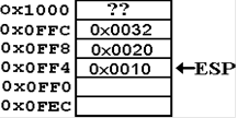
Suppose that the state of the stack before the invocation code for PROCA is as follows. We
assume that L, M, and N are passed by value and that L = 16 (0x10), M = 32 (0x20), and
N = 50 (0x32).

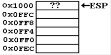ESP = 0x1000, pointing to something of
use in the calling routine.

Assume that the frame pointer for the calling
routine has the value
EBP = 0x100C.

We now show a possible assembly language version of the calling code. Note that the
addresses assigned to each instruction are only plausible.

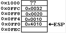
; PROCA (L, M, N)
0x4000   PUSH N
0x4004   PUSH M
0x4008   PUSH L
0x400C   CALL PROCA
0x4010   ADD ESP, 12

Here is a step by step illustration.

1. The passed arguments, if any, are pushed onto the stack.

2. The CALL instruction causes the return address to be pushed onto the stack.

At this point, we must consider a plausible assembly language representation of the procedure
PROCA. Note that the first line of code does not correspond to the first line in the high level
language. There is entry code to handle allocation on the stack. Here is some plausible code
for the first two lines of high level code.

;    INT PROCA (I, J, K)
     PUSH EBP
     MOV EBP, ESP    ; Give EBP a new value
     SUB ESP, 4     ; Set storage for a 4-byte local variable
     PUSH EAX         ; Save the value stored in EAX.

;    K1 = I + J + K
     MOV EAX,[EBP+8]
     ADD EAX,[EBP+12]   // Decimal values in source code
     ADD EAX,[EBP+16]
     MOV [EBP-4],EAX    // Store value in local variable

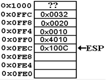
      3.   Before the execution of the first code in the subprogram, EBP is pushed onto the stack.
            This is done by the first assembly instruction in the entry code, which is PUSH EBP.
            Recall the assumed value for the base pointer EBP = 0x100C.

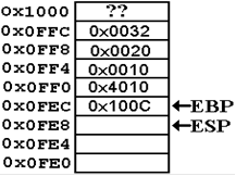
4. EBP is set to the value stored in ESP by the second line of the entry code,
MOV EBP,ESP. Now EBP = 0x0FEC.

5. Space is allocated on the stack to store any variables local to the subprogram. This is
done by the code SUB ESP, 4, which explicitly manipulates the stack.

At this point, note that the address of the local variable is given by [EBP – 4]. The addresses
of the three arguments (now called I, J, and K) are at [EBP +8], [EBP + 12], and [EBP + 16].

One of the standard assumptions about subprogram design is that subprograms do not have any
side effects. Possible side effects would include changing the values contained in any of the
general purpose registers, with the exception of ESP and EBP, which change by design. As
expected, the saved values are pushed onto the stack.

The subprogram sketched above is assumed to use only register EAX, and saves only that
register. Other subprograms may save all or none of the general purpose registers. At present,
when nobody codes in assembly language directly, it is the compiler conventions that dictate
what is stored on the stack.

6. The subprogram saves the value of EAX on the stack. At this point, the stack condition
is as follows.

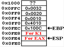Suppose that we are running a debugger and set the break
point at the first executable high level language instruction
K1 = I + J + K.

A simplistic reading of the textbooks indicates that the
stack pointer, ESP, should point to the return address. It
does not. The reason for this is that the entry code for the
subprogram has executed, and modified ESP.

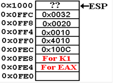
Exit Code for the Subprogram

The code for exiting any subprogram must undo the effects of the entry code. Here
are three lines that are typical of such exit code.

MOV ESP, EBP    // Set ESP to its value on entry, here 0x0FEC.
POP EBP         // Set EBP to its old value, here 0x100C.
                  // This sets ESP to 0x0FF0.
RET             // Pop return address from stack and return
                  // to address 0x4010. Now ESP = 0x0FF4.

The code at address 0x4010 completes the subroutine invocation by clearing the stack. The code
is ADD ESP, 12, which sets the stack pointer to ESP = 0x1000, the value before the code
sequence for the subprogram execution. Note the state of the stack after all this is done.

Here we see that nothing has been removed from the
actual memory. In the current designs, a stack POP will
not change the value in memory.

From a logical viewpoint, the memory at locations
0x0FE4 through 0x0FFF is no longer a part of the stack.

There are some security implications to leaving values in
memory, but we leave that to another course.

Stack Smashing

We now come to a standard trick used by malicious hackers. We shall define the term
by illustrating it. Suppose that our subprogram PROCA had, as its only local variable, an
array of four 32–bit integers. Call it A[4], with elements A[0], A[1], A[2], and A[3].

At the end of the entry code, the stack would resemble the following figure.

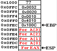The array A has only four elements, validly accessed
as A[0], A[1], A[2], or A[3]. Suppose that the high level
language lacks any array bounds checking logic. This
situation is common for many languages, as bounds
checking slows program execution.

Simply setting A[4] = 0 will wipe out the saved value
for EBP.

Setting A[5] = 0x2000 will change the return address.

This changing of non–data values on the stack is called
stack smashing. It has many malicious uses.

Static Code and Dynamic Data

It may or may not be true that the idea of using the stack for allocation of arguments, local
variables, and return addresses arose from the need to write recursive subprograms. While this
style of programming does facilitate recursion, indeed seeming to be necessary for it, it does
have more uses than that.

Another software design strategy requires what is called “reentrant code”, which is code that
can be invoked almost simultaneously by more than one program. Standard examples of this
style of coding are found in systems routines on time sharing computers.

Consider two users connected to the same computer and sharing its resources. A time sharing
operating system will allocate time to each user in turn, leaving each to assume that no other
users are accessing the computer. If these two users are both editing a file with the standard
editor, each will be using the same loaded code with different stack pointers.

In summary, the static allocation of data and return addresses does present some advantages
in execution speed. However, most users would prefer the flexibility afforded by dynamic
allocation, such as afforded by the stack and the heap.