Is
It Memory or an I/O Device?
There are two
ways of viewing a DASD, either as an extension of memory or as an
Input / Output device. Both views are
equally valid; the one to use depends on the feature
that is to be discussed. As a part of a
memory system, the disk plays a key role in virtual
memory. However, it is accessed as an
I/O device, and its interfacing must be discussed in
those terms. This textbook will discuss
disk drives a number of times.
Early
History of the Disk and Disk Drive
As noted earlier
in this textbook, data storage reached a crisis stage in the early 1950’s,
when the amount of physical floor space required to house the punched cards
holding the
data became excessive. The only option
was to develop new technology. IBM
addressed
the problem and delivered three new technologies: magnetic tape, the magnetic
drum, and
the magnetic disk. Each of these were
smaller and much faster to access than paper cards.
The first
magnetic tape drive was the IBM 729, released in 1952. While the dominant form
of secondary data storage for quite some time, magnetic tape drives are not
much used any
more. For that reason, we shall not
discuss magnetic tapes in any more detail.
The first
magnetic drum memory was the ERA 110, built for the U.S. Navy by Engineering
Research Associates of Minneapolis, MN.
The ERA 110 could store 1 million bits of
information, approximately 125 kilobytes.
One of the test engineers present at the first
sea trials of this device communicated the following to the author of this
textbook.
“The device spun at a high rate
in order to allow fast access to the data.
At first, the
trials were a success. When the ship
turned rapidly, the gyroscope effect took hold
and ripped the drive out of its mountings.”
Magnetic drum
memory was announced by IBM in 1953, and first shipped in 1954. While
the drum memory seemed to be a viable competitor for the magnetic disk, its
high cost and
low data density limited its use. The
only significant use by IBM for the drum memory was
as the main memory for the IBM 650, a first–generation computer announced in
July 1953
and last manufactured in 1962.
The RAMAC
The origin of
the magnetic disk drive was a research project started in 1952 by a group from
IBM in San Jose, CA. One of its main
goals was to develop a better technology for data
storage. Magnetic drums were considered,
but the choice was finally made to use a flat
platter design, as first reported by Jacob Rainbow of the National Bureau of
Standards (now
known as NIST) in 1952. The disk was
correctly assessed as having a bright future.
The first
commercial disk drive, called the RAMAC (Random–Access Method of
Accounting Control) 305 was demonstrated on September 13, 1956. The unit comprised
fifty aluminum disks of 24 inch diameter, coated on both sides with a magnetic
oxide
material that was a variant of the paint used on the Golden Gate Bridge.
The RAMAC 305
took up the better part of a room and could store all of 5MB of data -- the
equivalent of 64,000 punch cards or 2,000 pages of text with 2,500 characters
per page. The
drive system had an input/output data rate of roughly 10 kilobytes per second. It sold for
about $200,000 -- or you could lease it for about $3,200 a month. At that time, a good new
car from General Motors sold for about $2,000.
Here is an early picture of the RAMAC, taken from
the IBM archives. It is
physically a large unit.
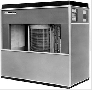
Figure: The Disks of the RAMAC 305
Later disk designs would all have at least one read/write
head for each recording surface, or
a pair of such heads for each
platter. The problem to be solved before
this innovation took
hold was how to suspend the heads
over the recording surface. The RAMAC
took a very
early approach, suggested probably
by the music “Juke Boxes” of the time.
It has one set
of two read/write heads that served
the entire drive.
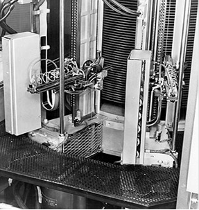
Figure:
The RAMAC Read/Write Heads
The
IBM 1301
The RAMAC 305
was the precursor to the IBM 1301 disk storage unit. When released in
1961, the 1301 was the first storage system that used "flying heads"
on actuator arms to read
and write data to its 50 24-inch magnetic platters. The 1301's head and
actuator arm
assembly looked something like a bread-slicing machine turned on its side
because
each drive platter had its own read/write head.
The 1301 had 13
times the capacity of the RAMAC, and its platters rotated at 1,800 rpm --
compared with a spindle speed of 100 rpm for the RAMAC -- allowing heads to
access the
data more quickly.
Only two years after
creating the 1301, IBM built the first removable hard drive, the 1311.
The drive system, which shrunk storage technology from the size of a
refrigerator to the size
of a washing machine, had six 14-inch platters and contained a removable disk
pack that had
a maximum capacity of 2.6MB of data. The 1311 remained in use through the
mid-1970s.
The concept of
integrating the disks and the head arm assembly as a sealed unit was
introduced by IBM with the “Winchester Drive” in 1973. Formally named the IBM 3340,
this drive had two spindles, each of 30 MB capacity; hence “30/30
Winchester”. Though a
project name, the term “Winchester” has been applied to the design
concept. Almost all
modern disk drives use the “Winchester design”.
While earlier designs provided for
removable disks, these allowed the disk to become dirty when exposed to the
outside air. In
the Winchester design, the entire assembly can be removed, thus keeping the
disks in a more
protected environment. With this higher
quality operating environment, the read/write heads
could be positioned closer to the disk platters, allowing for higher recording
densities.
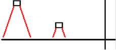
The relationship
between head flying height and track density can be seen in the rough
figure below. Each head will react to
tracks within a specific angular dimension; think of a
search light. The closer the head to the
recording surface, the smaller the spot containing
elements to which the head will react.
The head must not be able to react to more than one
data track at a time, hence its height dictates the minimum track spacing.
More Developments
In 1979, Al Shugart, who had helped develop the RAMAC with IBM,
launched Seagate
Technology Corp., which became the largest disk drive manufacturer in the
world. Soon
thereafter, the innovation floodgates opened. The "small form-factor"
hard drive was
invented in 1980 by Seagate. That five–inch
ST506 drive held the same capacity as the
RAMAC (5MB). From this point on, the
mass market associated with the newly arrived
PC (Personal Computer) movement guaranteed rapid evolution of the hard disk
drive.
History of Disk Costs
Here is a walk
through history [R030]. From the days of $10,000/MB to 2004 (from 2004 to
2009 the cost/GB has literally gone down to negligible levels), take a
look:
|
YEAR |
MANUFACTURER |
COST/GB |
|
1956 |
IBM |
$10,00,000 |
|
1980 |
North Star |
$193,000 |
|
1981 |
Morrow Designs |
$138,000 |
|
1982 |
Xebec |
$260,000 |
|
1983 |
Davong |
$119,000 |
|
1984 |
Pegasus (Great Lakes) |
$80,000 |
|
1985 |
First Class Peripherals |
$71,000 |
|
1987 |
Iomega |
$45,000 |
|
1988 |
IBM |
$16,000 |
|
1989 |
Western Digital |
$36,000 |
|
1990 |
First Class Peripherals |
$12,000 |
|
1991 |
WD |
$9,000 |
|
1992 |
Iomega |
$7,000 |
|
1994 |
Iomega |
$2000 |
|
1995 |
Seagate |
$850 |
|
1996 |
Maxtor |
$259 |
|
1997 |
Maxtor |
$93 |
|
1998 |
Quantum |
$43 |
|
1999 |
Fujitsu IDE |
$16 |
|
2000 |
Maxtor 7200rpm UDMA/66 |
$9.58 |
|
2001 |
Maxtor 5400 rpm IDE |
$4.57 |
|
2002 |
Western Digital 7200 rpm |
$2.68 |
|
2003 |
Maxtor 7200 rpm IDE |
$1.39 |
|
2004 |
Western Digital Caviar SE 7200rpm |
$1.15 |
More
recently disk prices have dropped even more.
In November 2007, the author of this
textbook purchased an external USB
500 GB disk drive for about $500.00 (or $0.50 per
gigabyte). On July 7, 2011, the web site for Office
Depot had the following prices:
a 500 GB USB external drive for $69.99 and a 1 TB USB external drive for
$119.99.
These prices are about five to seven cents per gigabyte.
We now
look at internal disk drives supporting the SATA standard. Also on July 7, 2011,
these prices were found. The WD Caviar Blue 500 GB drive with a 16 MB
buffer will sell
for $38.00 and the 3 TB WD Caviar
Green with a 64 MB buffer will sell for $140.
Do the math. This is very inexpensive.
How long
shall we have to wait for the first 1 petabyte drive?
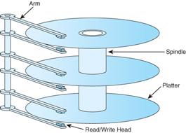
Structure of a Large Disk Drive
The typical large–capacity (and physically small) disk drive
has a number of glass platters
with magnetic coating. These spin at a high rate varying between
3,600 rpm (60/second)
and 15,000 rpm (250/second), with
7,200 rpm (120/second) being average. This
drawing
shows a disk with three platters and
six surfaces. In general, a disk drive
with N platters will
have 2·N surfaces, the top and bottom of
each platter.
On early disk drives, before the introduction of sealed
drives, the top and bottom surfaces
would not be used because they would
become dirty when the disk pack was removed.
The
introduction of the Winchester
design, with its sealed disks, changed that for the better.
More
on Disk Drive Structure
Each surface is divided into a number of concentric tracks. Each track has a number of
sectors. This figure shows an older style layout, in
which all tracks had the same number of
sectors. In such a design, the time for a sector to
move under the read/write head does not
depend on the track location,
simplifying the drive control logic.
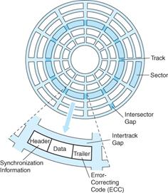
A sector usually contains 512 bytes of data, along with a
header and trailer part. Modern
designs have moved towards larger
sizes for sectors (say, 4,096) bytes, but the traditional
design has considerable history.
Modern
disk designs have divided the surface into a number of zones. This design is often
called ZBR (Zoned Bit Recording). Within each
zone, the sector count per track is
constant. However, the zones near the outer rim of the
disk have more sectors than the inner
zones. This increases the linear density of the
sectors for the outer zones, keeping that
density nearer that found in the
innermost zone, and making better use of the disk area.
Here is a picture of a disk surface
with color added to highlight the five zones.
Note that the
number of sectors per track
increases as we move from the inner zone to the outer zone.
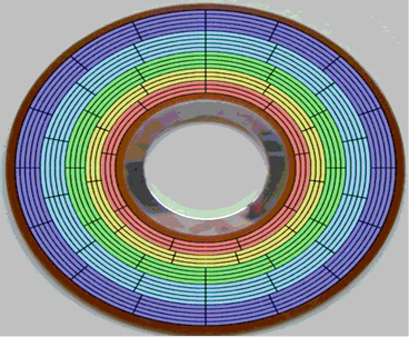
Figure:
Disk Surface with Five Zones
One downside to the ZBR strategy is that the complexity of
the disk–side controller must be
increased. In the older strategy, which might be called
one–zone, the sectors moved under
the read/write heads at the same
rate, without regard to track number. In
the above design,
the rate is constant within each zone,
but the controller must allow for five distinct rates.
Given the ability to fabricate
complex electronics, this is deemed a fair trade–off.
The
Disk Surface
The standard definition of a hard
disk drive is quite simple.
“The
recording medium for hard disk drives is basically a very thin layer of
magnetically hard material on a
rigid substrate.” [R031]
Up to the mid 1990’s, aluminum was used exclusively for the
substrate. Recently, glass has
attracted interest for a substrate,
mostly for its ability to be polished to a very fine surface
finish. Remember that the design goal is to reduce
the flying height of the read/write heads,
and that requires a smoother surface
over which to fly.
Since the earliest designs, each recording surface of a disk
has been divided into concentric
circles, called tracks. Optical disks, such as CDs and DVDs, as well
as vinyl records, have a
single spiral track on each
recording surface. According to Jacob [R008]
“The
major reasons for this are partly historical … In the early days of disk
drives, when open–loop mechanical
systems were used to position the head,
using concentric tracks seemed a
natural choice. Today, the closed–loop
embedded servo system … makes spiral
track formatting feasible. Nonetheless
concentric tracks are a
well–understood and well–used technology and seem
easier to implement than spiral
tracks.”
Timing
of a Disk Transfer
Disks are electromechanical devices. The time for a data transfer has a number of
components, including time to decode
the command, time to move the read/write heads to
the proper location on the disk,
time to transfer the data to the on–disk data buffers, and time
to transfer the data across the
interface to the host–side interface.
Here, we consider two of
the more important disk timings:
seek time and rotational latency.
The idea of seek time
reflects the fact that, in order to access a disk track for either a read or
write operation, the heads must be
moved to the track. This is a mechanical
action, as the
read/write heads are physical
devices. Some early designs seem to have
avoided this
problem by having one read/write
head per track. This is not an option
for modern drives,
which have thousands of tracks per
surface.
There are two seek times typically quoted for a disk.
Track–to–track: the time to move the heads to the
next track over
Average: the average time to move
the heads to any track.
The rotational delay is due to the fact that the disk is spinning
at a fixed high speed. It takes
a certain time for a specific sector
to rotate under the read/write heads. Suppose
a disk
rotating at 12,000 RPM. That is 200 revolutions per second. Each sector moves under the
read/write heads 200 times a second,
once every 0.005 second or every 5 milliseconds. The
rotational
latency, or average rotational delay, is
one half of the time for a complete
revolution of the disk. Here it would be 2.50 milliseconds.
Rotational latency is a major component of the time to
access data on a disk. For that
reason, methods to minimize the
rotational latency of a disk are under active investigation.
One way would be to speed up the
rotation of the disk. Unfortunately, this
leads to stress on
the physical platters that become
unacceptable. This is seen in a design
choice for the 5¼
floppy drives, which were spun at a
leisurely 360 rpm. The reason for this
rate is that a
significantly higher rate would cause
the disks to be torn apart by centrifugal forces.
Another method to reduce rotational latency would be to add
a second actuator with its own
set of read write heads to the disk
drive. This would be positioned opposite
the first set.
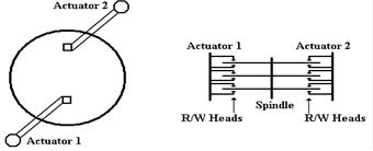
Figure: Two
Views of Dual Actuators
Such a design would immediately halve the rotational
latency, as the average time for a
sector to move under one of the
read/write heads would be one quarter of a revolution. For a
12,000 rpm disk, the rotational
delay would be cut from 2.50 to 1.25 milliseconds. Put
another way, the reduction is from
2, 500, 000 nanoseconds to 1, 250, 000 nanoseconds.
However, the addition of a second
set of heads raises the price by about 35%, not acceptable
in the highly competitive modern
market. Conner Peripherals introduced
such a product in
1994, but it was not popular. The design has never been attempted since.
Tracks and Cylinders
The idea of a cylinder is an artifact of the mechanical
nature of the actuators used to move
the read/write heads on a modern
disk. It is faster to read sectors from
the same track than it
is to move to another track, even
one close by. We now consider the fact
that standard disk
drives with concentric tracks and
multiple recording surfaces have the same number of
tracks and track geometry on each of
the surfaces.
When the actuator is functioning properly, as it almost
always is, each read/write head is
over (or near to) the same numbered
track on its disk. This leads to the
idea of a cylinder as
the set of tracks that can be read
without significant repositioning of the read/write heads. In
early disk designs, with wider
tracks, there would be no positioning required to move from
surface to surface on a
cylinder. All that would be required was
an electronic switching of
the active head, a matter of
nanoseconds and not milliseconds.
We close this
part of the chapter with some related questions. How many bytes of data can
be read from a disk before the read/write heads must be moved? What is the maximum data
transfer rate from a multi–platter disk?
How long can this rate be sustained?
Disk Capacity
The first
question is how to calculate the capacity of a disk. Here are a number of
equivalent ways, assuming the standard 512 bytes per sector.
Disk Capacity = (number of surfaces)·(bytes per
surface)
= (number of surfaces)·(tracks per
surface)·(bytes
per track)
= (number of surfaces)·(tracks per
surface)·
(sectors per track)·512
Here are data
from an earlier disk drive (now rather small).
8 surfaces
3196 tracks per
surface
132 sectors per
track
512 bytes per
sector
Surface
capacity = 3196·132·512 = 421872·512 = 210936·1024 bytes
= 210936 KB » 206.0 MB
Disk
capacity = 8·210936 KB = 1,687,488 KB »
1.61 GB
Computing Disk Maximum Transfer Rate
We now compute
the maximum transfer rate. This is
computed from the size of a track in
bytes and the rotation rate of the disk.
For modern disks, the transfer rate would depend on
the zone in which the track is located, as each zone has a different number of
sectors per
track. For this example, we use the
older disk with only one track size.
Disk rotation
rates are given in RPM (Revolutions per Minute). Common values are 3,600
RPM, 7,200 RPM, and higher. 3,600 RPM is
60 revolutions per second. 7,200 PRM is
120 per second. Consider our sample
disk. Suppose it rotates at 7,200 RPM,
which is
one revolution every (1/120) second.
One track contains 132·512 bytes = 66·1024 bytes =
66KB.
This track can be read in
(1/120) of a second.
The maximum data rate is 66 KB in (1/120) of a second.
120
·
66 KB in one second.
7,920
KB per second = 7.73 MB per second.
Sustaining the
Maximum Data Transfer Rate
Recall the
definition of a cylinder as a set of tracks, one per surface. Each track can be read
in one revolution of the disk drive. The
data rate can be sustained for as long as it takes to
read all tracks from the cylinder.
The number of
tracks per cylinder is always exactly the same as the number of surfaces in
the disk drive. Our sample drive has 8
surfaces; each cylinder has 8 tracks.
In our sample
drive, rotating at 7200 RPM or 120 per second:
Each track can be
read in 1/120 second.
The cylinder,
containing 8 tracks, is read in 8/120 second or 1/15 second.
The maximum data
transfer rate can be sustained for 1/15 second.
How Much Data
Can Be Transferred at This Rate?
Each track can
be read in 1/120 of a second. The
cylinder can be read in 1/15 second.
The cylinder contains 8 tracks of 66·1024 bytes, thus
8·66·1024 = 528 KB.
The Drive Cache
Modern disk
drives have a cache memory associated with the on–disk controller. Some
manufacturers call this a “databurst
cache”. On modern drives, this can
vary between
2 MB and 64 MB; DRAM is quite cheap these days.
The disk–side
cache grew out of the small disk–side data buffers required to match the speed
of the disk internal transfers with the speed of the bus connecting it to the
controller logic on
the host side. Buffering is also
required in those cases when the interface to the host is busy
at the time the disk read/write heads are ready to initiate a transfer. On a disk write, the host
controller would transfer the data to the disk–side buffer for later writing to
the disk itself.
As DRAM prices
dropped, this simple data buffer grew into a full–fledged cache. The
utility of this cache does not depend on a high hit rate, as it does for the
cache between
primary memory and the CPU. One of its
main uses is in allowing the disk controller to
prefetch data; that is, to copy the data into the buffer before it is
requested. This increases
the efficiency of disk reads. As a write
buffer, the cache speeds up disk writes.
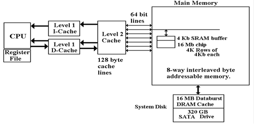
We now have
quite a few levels of cache memory between the disk surfaces and the CPU.
Here is a diagram showing the configuration on a computer built in 2007. The disk has a
16 MB DRAM cache. Each memory chip has a
4 Kb (kilobit) SRAM buffer. There are
two
levels of cache between the main memory and the CPU.
The
Disk Directory Structure
We now turn our
attention to the disk directory structure.
Rather than discussing the more
modern structures, such as NTFS, we shall limit ourselves to older and simpler
structures.
The
FAT (File Allocation Table)
Physically the
disk contains a large number of sectors, each of which contains either data or
programs. Logically the disk contains a
large number of files, also program and data.
The
disk will have one or more index structures that associate files with their
sectors.
The two important structures are
the disk directory associates a file with its
first sector
the File Allocation Table maintains the “linked list” of sectors
for that file.
This example shows
the structure of the FAT.
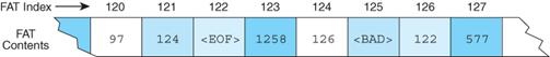
Here
the disk directory indicates that the first sector for a file is at address
121.
The
FAT entry at 121 indicates that the next sector is at address 124.
The
FAT entry at 126 indicates that the next sector is at address 122.
The FAT entry at
122 indicates that sector 122 is the last for this file. Sector 125 is bad.
The FAT–16
system was implemented by Microsoft for early versions of MS–DOS. This
system used a 16–bit index into the FAT.
As there is one FAT entry per sector, this makes
this limits the sector count to 216.
The maximum disk size is thus 216· 512 = 216· 29 =
225 =
25· 220 = 32 MB. In 1987, my brand–new PC/XT had a 20MB
disk! FAT–16 worked very
well. What about a 40 MB disk? How about a 256 MB disk?
Few people in
the late 1980’s contemplated disk drives with capacities of over 100 GB,
but it was obvious that unmodified FAT–16 would not do the job. We consider two short–
term remedies to this problem, one transient and one with longer term
consequences.
The first
solution was to partition a larger physical disk drive into two logical disk
drives.
A 40 MB disk
drive would support two logical disks, each with its own directory structure
and File Allocation Table. Using the
drive names suggested at the time, this 40 MB
physical disk would support two logical disks: Drive C with capacity of 32 MB,
and
Drive D with capacity of 8 MB.
As a short–term
fix, this worked well. However, it just
raised the limit to 64 MB. This
solution was obsolete by about 1992. The
main problem with the FAT–16 system arose
from the fact that each sector was individually addressable. With 216 addresses available,
we have a maximum of 216 sectors or 32 MB for each logical drive.
The second
solution was to remove the restriction that each sector be addressable. Sectors
were grouped into clusters, and only clusters could be addressed. The number of sectors a
cluster contained was constrained to be a power of 2; so we had 2, 4, 8, 16,
etc. sectors per
cluster. The effect on disk size is easy
to see.
|
Sectors in Cluster |
1 |
2 |
4 |
8 |
16 |
32 |
64 |
|
Bytes in Cluster |
512 |
1024 |
2048 |
4096 |
8192 |
16384 |
32768 |
|
Disk Size |
32 MB |
64 MB |
128 MB |
256 MB |
512 MB |
1 GB |
2 GB |
In the early 1990’s, it seemed that this solution
would work for a while. Nobody back then
envisioned multi–gigabyte disk drives on personal computers. There is a problem associated
with large clusters; it is called “internal
fragmentation”.
This problem
arises from the fact that files must occupy an integer number of clusters.
Consider a data
file having exactly 6,000 bytes of data, with several cluster sizes.
|
Sectors in Cluster |
1 |
2 |
4 |
8 |
16 |
32 |
64 |
|
Bytes in Cluster |
512 |
1024 |
2048 |
4096 |
8192 |
16384 |
32768 |
|
Clusters needed |
12 |
6 |
3 |
2 |
1 |
1 |
1 |
|
File size on disk |
6144 |
6144 |
6144 |
8192 |
8192 |
16384 |
32768 |
|
Disk efficiency |
97.7% |
97.7% |
97.7% |
73.2% |
73.2% |
36.6% |
18.3% |
Security Issues: Erasing and Reformatting
Remember the
disk directory and the FAT. What happens
when a file is erased from the
disk? The data are not removed. Here is what actually happens.
1. The file name is removed from the disk directory.
2. The FAT is modified to place all the sectors (clusters) for
that file
into a special
file, called the “Free List”.
3. Sectors do not have their data erased or changed until they
are allocated
to another file
and that a program writes data to that file.
For this reason, many companies sell utilities to
“Wipe the File” or “Shred the File”.
How about reformatting the disk? Certainly, that removes file links. Again the data are not
removed. The directory structure and FAT
are reinitialized and the free list reorganized.
The sectors containing the data are not overwritten until they are reused.
Interfaces
to Disk Drives
The disk drive
is not a stand–alone device. In order to
function as a part of a system, the disk
must be connected to the motherboard through a bus. We shall discuss details of disk drives in
the next chapter. In this one, we focus
on two popular bus technologies used to interface a disk:
ATA and SATA. Much of this material is
based on discussions in chapter 20 of the book on
memory systems by Bruce Jacob, et al [R008].
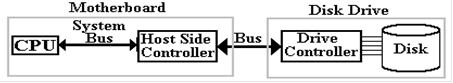
The top–level
organization is shown in the figure below.
We are considering the type of bus
used to connect the disk drive to the motherboard; more specifically, the host
controller on
the motherboard to the drive controller on the disk drive. While the figure suggests that the
disk is part of the disk drive, this figure applies to removable disks as
well. The important
feature is the nature of the two controllers and the protocol for
communication.
One of the
primary considerations when designing a disk interface, and the bus to implement
that
interface, is the size of the drive controller that is packaged with the
disk. Jacob [R008] noted:
“In the early days, before Large
Scale Integration (LSI) made adequate computational
power economical to be put in a disk drive, the disk drives were ‘dumb’
peripheral
devices. The host system had to
micromanage every low–level action of the disk drive.
… The host system had to know the detailed physical geometry of the disk drive;
e.g.,
number of cylinders, number of heads, number of sectors per track, etc.”
“Two things changed this
picture. First, with the emergence of
PCs, which eventually
became ubiquitous, and the low–cost disk drives that went into them, interfaces
became
standardized. Second, large–scale
integration technology in electronics made
it economical to put a lot of intelligence in the disk side controller”
As of Summer
2011, the four most popular interfaces (bus types) were the two varieties of
ATA
(Advanced Technology Attachment, SCSI (Small Computer Systems Interface), and
the FC
(Fibre Channel).
The SCSI and FC interfaces are more costly, and are commonly used on
more
expensive computers where reliability is a premium. We here discuss the two ATA busses.
The ATA
interface is now managed by Technical Committee 13 of INCITS (www.t13.org), the
International Committee for Information Technology Standards
(www.incits.org). The interface
was so named because it was designed to be attached to the IBM PC/AT, the
“Advanced
Technology” version of the IBM PC, introduced in 1984. To quote Jacob again:
“The first hard disk drive to be
attached to a PC was Seagate’s ST506, a 5.25 inch form
factor 5–MB drive introduced in 1980.
The drive itself had little on–board control
electronics; most of the drive logic resided in the host side controller. Around the second
half of the 1980’s, drive manufacturers started to move the control logic from
the host side
and integrate it with the drive. Such
drives became known as IDE (Integrated Drive
Electronics) drives.”
In recent years,
the ATA standard has being explicitly referred to at the “PATA” (Parallel ATA)
standard to distinguish it from the SATA (Serial ATA standard) that is now
becoming popular.
The original PATA standard called for a 40–wire cable. As the bus clock rate increased, noise
from crosstalk between the unshielded cables became a nuisance. The new design included
40 extra wires, all ground wires to reduce the crosstalk.
As an example of
a parallel bus, we show a picture of the PDP–11 Unibus. This had 72 wires, of
which 56 were devoted to signals, and 16 to grounding. This bus is about 1 meter in length.
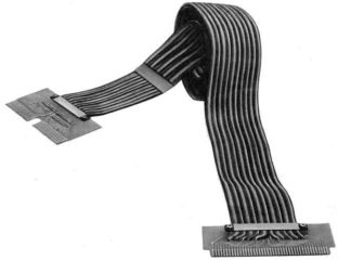
Figure: The Unibus of the PDP–11 Computer
Up to this
point, we have discussed parallel busses.
These are busses that transmit N data bits
over N data lines, such as the Unibus™ that used 16 data lines to transmit two
bytes per transfer.
Recently serial busses have become popular; especially the SATA (Serial
Advanced Technology
Attachment) busses used to connect internally mounted disk drives to the motherboard. There
are two primary motivations for the development of the SATA standard: clock
skews and noise.
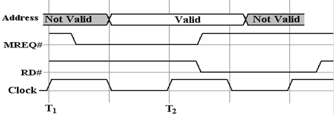
The problem of
clock skew is illustrated by the following pair of figures. The first figure shows
a part of the timing diagram for the intended operation of the bus. While these figures may be
said to be inspired by actual timing diagrams, they are probably not realistic.
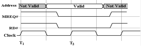
In the above figure, the control signals MREQ# and RD# are
asserted simultaneously one half
clock time, after the address
becomes valid. The two are
simultaneously asserted for two clock
times, after which the data are
read.
We now imagine what could go wrong when the clock time is
very close to the gate delay times
found in the circuitry that
generates these control signals. For
example, let us assume a 1 GHz
bus clock with a clock time of one
nanosecond. The timing diagram above
calls for the two
control signals, MREQ# and RD#, to
be asserted 0.5 nanoseconds (500 picoseconds) after the
address is valid. Suppose that the circuit for each of these is
skewed by 0.5 nanoseconds, with
the MREQ# being early and the RD#
being late.
What we have in this diagram is a mess, one that probably
will not lead to a functional read
operation. Note that MREQ# and RD# are simultaneously
asserted for only an instant, far too
short a time to allow any operation
to be started. The MREQ# being early may
or may not be a
problem, but the RD# being late
certainly is. A bus with these skews
will not work.
As discussed above, the ribbon cable of the PATA bus has 40
unshielded wires. These are
susceptible to cross talk, which
limits the permissible clock rate. What
happens is that crosstalk
is a transient phenomenon; the bus
must be slow enough to allow its effects to dissipate.
We have already seen a solution to the problem of noise when
we considered the PCI Express
bus.
This is the solution adopted by the SATA bus. The standard SATA bus has a seven–wire
cable for signals and a separate
five–wire cable for power. The seven–wire
cable for data has
three wires devoted to ground (noise
reduction) and four wires devoted to a serial lane, as
described above for PCI
Express. As noted above in that
discussion, the serial lane is relatively
immune to noise and crosstalk, while
allowing for very good transmission speeds.
One might note that parallel busses are inherently faster
than serial busses. An N–bit bus will
transmit data N times faster than a
1–bit serial bus. The experience seems
to be that the data
transmission rate can be so much
higher on the SATA bus than on a parallel bus, that the SATA
bus is, in fact, the faster of the
two. Data transmission on these busses
is rated in bits per second.
In 2007, according to Jacob [R008]
“SATA controllers and disk drives with 3 Gbps are starting
to appear, with 6 Gbps on SATA’s
roadmap.” The encoding used is called
“8b/10b”, in which
an 8–bit byte is padded with two error correcting bits to be transmitted as 10
bits. The two
speeds above correspond to 300 MB
per second and 600 MB per second.