The Evolution of Microprogramming
In this lecture, we deviate somewhat from the textbook
and discuss the history of microprogrammed control
units.
The main topics for this lecture are as follows:
1. A review of the function of the Control Unit
as a part of
the CPU and the standard ways to
implement control.
2. A quick introduction to VHDL, a language that
can be
used to design and test a
hardwired control unit.
3. The origin of the microprogrammed control
unit, and
factors that affected its early
development.
We
begin with a review of the CPU (Central Processing Unit) of a typical computer,
and comment on function of the control unit.
The Central Processing Unit (CPU)
The CPU has four main components:
1. The
Control Unit (along with the IR) interprets the machine language instruction
and issues the control signals to
make the CPU execute that instruction.
2. The
ALU (Arithmetic Logic Unit) that does the arithmetic and logic.
3. The
Register Set (Register File) that stores temporary results related to the
computations. There are also Special Purpose Registers used by the Control Unit.
4. An
internal bus structure for communication.
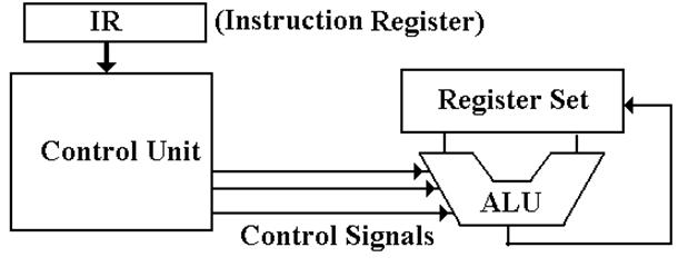
The
function of the control unit is to
decode the binary machine word in the IR (Instruction Register)
and issue appropriate control signals, mostly to the CPU. It is the control signals that cause the
computer to execute its program.
Design of the Control Unit
There are two related issues when considering the
design of the control unit:
1) the complexity of the
Instruction Set Architecture, and
2) the microarchitecture
used to implement the control unit.
In order to make decisions on the complexity, we must
place the role of the control unit within the
context of what is called the DSI (Dynamic Static Interface).
The ISA (Instruction Set Architecture) of a
computer is the set of assembly language commands that
the computer can execute. It can be seen
as the interface between the software (expressed as
assembly language) and the hardware.
A more complex ISA requires a more complex control
unit.
At some point in the development of computers, the
complexity of the control unit became a problem
for the designers. In order to simplify
the design, the developers of the control unit for the IBM–360
elected to make it a microprogrammed
unit.
We shall spend some time investigating the motivations
of the IBM design team.
The Dynamic–Static Interface
In order to understand the DSI, we must place it
within the context of a compiler for a higher–level
language. Although most compilers do not
emit assembly language, we shall find it easier to
under the DSI if we pretend that they do.
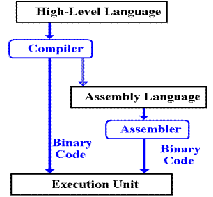
What does the compiler output? There are two options:
1. A very simple assembly language. This requires a sophisticated compiler.
2. A more
complex assembly language. This may
allow a simpler compiler,
but it requires a more complex
control unit. If complex enough, parts
of the
control unit are probably
microprogrammed.
How Does the
Control Unit Work?
The binary form of the instruction is now in the IR (Instruction Register).
The control unit decodes that instruction and
generates the control signals necessary for the CPU
to act as directed by the machine language instruction.
The two major design categories here are hard–wired and microprogrammed.
Hardwired: The control signals are
generated as an output of a
set
of basic logic gates, the input of which derives
from
the binary bits in the Instruction Register.
Microprogrammed: The control signals
are generated by a microprogram
that
is stored in Control Read Only Memory.
The
microcontroller fetches a control
word from the
CROM and places it into the mMBR, from which
control
signals are emitted.
The
microcontroller can almost be seen as a very simple computer within a more
complex computer.
This simplicity was part of the original motivation.
The Microprogrammed
Control Unit
In
a microprogrammed control unit, the control signals correspond to bits in a micromemory (CROM
for Control ROM), which are read
into a micro–MBR. This register is just
a set of D flip–flops,
the contents of which are emitted as signals.
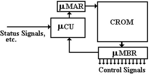
The micro–control unit ( mCU )
1) places
an address into the micro–Memory Address Register ( mMAR ),
2) the
control word is read from the Control Read–Only Memory,
3) puts
the microcode word into the micro–Memory Buffer Register, and
4) the
control signals are issued.
Maurice Wilkes
Maurice Wilkes worked in the Computing Laboratory at
Cambridge University beginning in 1936,
but mostly from 1945 as he served in WW 2.
He read von Neumann’s preliminary report on the EDVAC
in 1946. He immediately “recognized
this as the real thing” and started on building a stored program computer. In August 1946 he attended
a series of lectures “Theory and Techniques for Design of Electronic Digital
Computers” given at the
Moore School of Engineering at the University of Pennsylvania and met many of
the designers of the ENIAC.
On May 6, 1949 the EDSAC was first operational,
computing the values of N2 for
1 £ N £ 99. In 1951, Wilkes
published The Preparation of Programs for Electronic Digital Computers,
the first book on programming. I have a
1958 edition.
Also in 1951, Wilkes published a paper “The Best Way
to Design an Automatic Calculating Machine”
that described a technique that he microprogramming. This technique is still in use today and
still
has the same name.
In 1953, Wilkes and Stringer further described the
technique and considered issues of
design complexity, test and verification of the control logic, pipelining
access to the
control store, and support of different ISA (Instruction Set Architectures)
(Wilkes and Stringer, 1953).
Wilkes’ Motivations
“As soon as we started programming, we found to our
surprise that it wasn’t as easy to get
programs right as we had thought. … I can remember the exact instant when I
realized that a
large part of my life from then on was going to be spent in finding mistakes in
my own programs.”
After his visit to the United States, Wilkes started
to worry about the complexity of the control unit of the
EDVAC, then in design. Here is what he
wrote later.
“I found that it did indeed have a
centralized control based on the use of a matrix of diodes. It was,
however, only capable of producing a fixed sequence of eight pulses—a
different sequence for each
instruction, but nevertheless fixed as far as a particular instruction was
concerned. It was not, I think,
until I got back to Cambridge that I realized that the solution was to turn
the control unit into a
computer in miniature by adding a second matrix to determine the flow of
control at the microlevel
and by providing for conditional microinstructions.”
In other words, have the control signals emitted by a
smaller computer that is controlled by a microprogram.
The advantage is that the control unit of this smaller computer is extremely
simple to design, test, and understand.
A Diode Memory
A diode is a one way current gate. It causes current to flow one way only.
Specifically: For
current in one direction, it offers almost no resistance
For
current in the opposite direction, it appears as a very large resistance.
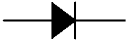
A diode memory is just a collection of diodes
connected in a matrix.
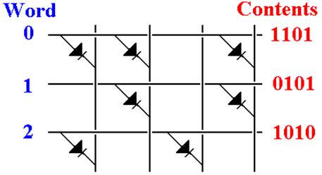
Follow
the current paths. This shows the
contents of each word. This is a classic
ROM.
Problems in the 1950’s
In 1958, the EDSAC 2 became operational; it was the
first microprogrammed computer.
The control unit used ROM made from magnetic cores (Hennessy & Patterson,
1990).
There were two reasons that Wilkes’ idea did not take
off in the 1950’s.
1. The simple instruction sets of the time did
not demand microprogramming, and
2. The methods for fabricating a microprogram
control store were not adequate.
All of this changed when IBM embraced microprogramming
as a method for the
control units of their System/360 design.
We should note that the early control stores for the
IBM System/360 were implemented
with technologies that are no obsolete and strange to our ears.
BCROS Balanced Capacitor Read–Only Storage
Two capacitors per
word in a storage of 2816 words of 100 bits each.
TROS Transformer
Read–Only Storage.
Magnetic core
storage of 8192 words of 54 bits each.
CCROS Card Capacitor
Read–Only Storage.
Mylar cards the
size of standard punch cards with copper tabs.
Early Interest in Microprogramming
We begin by quoting from the article Readings in Microprogramming.
“Microprogram control is seen as a form of simulation
in which
primitive operations are combined and sequenced so as to imitate
the characteristics of a desired machine.”
Davies begins his article with a discussion of what
then was an important use
of microprogramming – to use one computer to emulate another.
He considers two incompatible architectures: the IBM
7040 and IBM 7094.
He postulated the following scenario.
1. There is at hand an IBM 7094 upon which we
want to run a program.
This will be called the host system.
2. There is a large [assembly language] program
written for an IBM 7040.
This is called the target system.
The IBM 7094 running IBM 7040 code is called a virtual system.
Source: (Davies, 1972)
Microprogramming is Taken Seriously
It was with the introduction of the IBM System/360
that microprogramming was taken
seriously as an option for designing control units. There were three reasons.
1. The recent availability of memory units with
sufficient reliability and
reasonable cost.
2. The fact that IBM took the technology
seriously.
3. The fact that IBM aggressively pushed the
memory technology inside the
company to make microprogramming
feasible.
IBM’
goals are stated in the 1967 paper by Tucker.
“Microprogramming in the System/360 line is not meant
to provide the problem programmer
with an instruction set that he can custom–tailor. Quite the contrary, it has been used to help
design a fixed instruction set capable of reaching across a compatible line of
machines in a wide
range of performances. … The use of microprogramming has, however, made it
feasible for the
smaller models of System/360 to provide the same comprehensive instruction set
as the large models.”
Tucker notes that the use of a ROS
[Read Only Store] is somewhat expensive, becoming attractive
only as “an instruction set becomes more comprehensive”.
Source: (Page 225 of Tucker, 1967)
Microprogramming is Taken Seriously
(By IBM’s Customers)
The primary intent of the IBM design team was to
generate an entire family of computers with one
ISA (Instruction Set Architecture) but many different organizations.
Microprogramming allowed computers of a wide range of
computing power (and cost)
to implement the same instruction set and run the same assembly language
software.
Several of the IBM product line managers saw another
use for microprogramming, one that their
customer base thought to be extremely important: allowing assembly language
programs from
earlier models (IBM 1401, IBM 7040, IBM 7094) to run
unchanged
on any model of the System/360 series.
As one later author put it, it was only the
introduction of microprogramming and the emulation of
earlier machines allowed by this feature that prevented “mass defections” of
the IBM customer base
to other companies, such as Honeywell, that were certainly looking for the
business.
This idea was proposed and named “emulation” by Stewart Tucker (quoted above).
The 1960’s and 1970’s
Here I just quote our textbook.
“In the 1960s and 1970s, microprogramming
was one of the most important techniques used in
implementing machines. Through most of that period, machines were implemented
with discrete
components or MSI (medium-scale integration—fewer than 1000 gates per chip), ….[Designers
could choose between a hardwired control unit based on a finite–state–machine
model or a
microprogrammed control unit].
The reliance on standard parts of low- to
medium-level integration made these two design styles
radically different. Microprogrammed approaches were attractive because
implementing the control
with a large collection of low-density gates was extremely costly. Furthermore,
the popularity of
relatively complex instruction sets demanded a large control unit, making a
ROM-based implementation
much more efficient. The hardwired implementations were faster, but too costly for
most machines.
Furthermore, it was very difficult to get the control correct, and changing
ROMs was easier than
replacing a random logic control unit. Eventually, microprogrammed control was
implemented in RAM,
to allow changes late in the design cycle, and even in
the field after a machine shipped.”
The Microprogram Design Process
Here we make an assertion that is almost true on the
face of it: the design and testing of a control unit is
one of the more difficult parts of developing a new computer.
In the late 1970’s, microprogramming had become popular. One of the reasons was the way in which it
facilitated the process of designing the
control unit.
Microprogramming was quite similar to assembly
language programming;
many designers of the time were experts at this.
Microprogram assemblers had been developed and were in
wide use.
The process of microprogram development was simple:
1. Write the microcode in a symbolic “microassembly”
language and assemble it into
binary microcode.
2. Download the microcode to an EPROM (Erasable
Programmable ROM) using a ROM
programmer.
3. Test the microcode, fix the problems, and
repeat.
The Hardwired Control Unit Design Process
In contrast, prototyping a hardwired control unit took
quite a bit of effort. The unit was
built from LSI
and MSI components, wired and tested.
This was very labor intensive and costly, since it most of the
work had to be done by degreed engineers.
Recall that in the 1970’s there were few tools to aid
hardware design. In particular, there
were no
programmable gate arrays to allow quick configuration of hardware and no
hardware design languages,
such as VHDL, for describing and testing a design.
Today, a hardwired control unit is as easy to design
and test as a microprogrammed unit;
it is first described and tested in VHDL.
Source: Page
189 from (Murdocca, 2007)
Benefits of Microprogramming
As noted above, the primary impediment to adoption of
microprogramming was that
sufficiently fast control memory was not readily available.
When the necessary memory became available,
microprogramming became popular.
The main advantage of microprogramming was that it
handled difficulties associated
with virtual memory, especially those of restarting instructions after page
faults.
The IBM System 370 Model 138 implemented virtual
memory entirely in microcode
without any hardware support (Hennessy & Patterson, 1990).
Here is a personal memory, dating from the early
1980’s. At that time computers for the
direct execution of the LISP programming language were popular, and there were
two
major competitors: Symbolics and LMI.
At a meeting in
Early in the competition, the LMI – 1 had fared poorly, running at about half
of the speed
of the Symbolics –3670. The LMI engineers immediately redesigned the
control store
to execute code found in the benchmark.
By the competition, the LMI – 1 was officially
a bit faster than the Symbolics – 3670.
The IBM XT/370
IBM was attempting to regain dominance in the desktop
market.
They noted that both the S/370 and the Motorola 68000
used sixteen 32–bit general purpose registers.
In 1984 IBM announced the XT/370, a “370 on a
desktop”, a pair of Motorola 68000s re–microprogrammed
to emulate the S/370 instruction set.
Two units were required because the control store on the Motorola
was too small for the S/370.
As a computer the project was successful. It failed because IBM wanted full S/370
prices for the
software to run on the XT/370.
Source: Page
189 from (Murdocca, 2007)
Confirmed on the IBM Web Site (Kozuh, 1984)
Side–Effects of Microprogramming
It is a simple fact that the introduction of
microprogramming allowed the development of Instruction Set
Architectures of almost arbitrary complexity.
The VAX series of computers, marketed by the Digital
Equipment Corporation, is usually seen as the
“high water mark” of microprogrammed designs.
The later VAX designs supported an Instruction Set
Architecture with more than 300 instructions and more than a dozen addressing
modes.
When examining the IA–32 Instruction Set Architecture,
we may not a number of instructions of significant
complexity. These were introduced to
support high–level languages (remember the “semantic gap”). It was
later discovered that these were rarely used by compilers, but the “legacy
code” issue forced their retention.
It is now the case that the existence of these
instructions in the IA–32 ISA required that part of the control
unit be microprogrammed; a hardwired control unit would be too complex. The ghost of the Intel 80286 still haunts us.
VHDL
The VHDL was proposed in the late 1980’s (IEEE
Standard 1076–1987) and refined in the 1990’s
(IEEE Standards 1164 and 1076–1993). The
term VHDL stands for
VHSIC (Very High Speed Integrated Circuits) Hardware Description Language.
Here is the VHDL description of a two–input AND gate.
entity AND2 is
port
(in1, in2: in std_logic;
out1:
out std_logic);
end AND2;
architecture
behavioral_2 of AND2 is
begin
out1 <= in1
and in2;
end behavioral_2;
Microprogramming and Memory Technologies
The drawback of microcode has always been memory performance;
the CPU
clock cycle is limited by the time to read the memory.
In the 1950’s, microprogramming was impractical for
two reasons.
1. The memory available was not reliable, and
2. The memory available was the same slow core
memory as used in
the main memory of the computer.
In the late 1960’s, semiconductor memory (SRAM) became
available for the
control store. It was ten times faster
than the DRAM used in main memory. It
is this speed difference that opened the way for microcode.
In the late 1970’s, cache memories using the SRAM
became popular. At this
point, the CROM lost its speed advantage.
“For these reasons, instruction sets
invented since 1985 have not relied on
microcode” (Hennessy & Patterson, 1990).
Microprogramming: The Late Evolution
“The Mc2 [microprogramming control] level was the
standard design for practically all commercial
computers until load/store architectures became fashionable in the 1980s”.
Events that lead to the reduced emphasis on
microprogramming include:
1. The availability of VLSI technology, which
allowed a number of improvements,
including on–chip cache memory,
at reasonable cost.
2. The availability of ASIC (Application
Specific Integrated Circuits) and FPGA
(Field Programmable Gate
Arrays), each of which could be used to create
custom circuits that were easily
tested and reconfigured.
3. The beginning of the RISC (Reduced
Instruction Set Computer) movement, with
its realization that complex
instruction sets were not required.
Modern design practice favors a “mixed control unit”
with hardwired control for the simpler (and more
common) instructions and microcode implementation of the more complex (mainly
legacy code) instructions.
The later versions (80486 and following) of the Intel
IA–32 architecture provide a good example of
this “mixed mode” control unit. We
examine these to close the lecture.
(page 618 of Warford, 2005)
The IA–32 Control Unit
In order to understand the IA–32 control unit, we must
first comment on a fact of instruction
execution in the MIPS. Every instruction
in the MIPS can be executed in one pass through
the data path. What is meant by that?
In this chapter, we have studied two variants of the
MIPS data path.
1. A single–cycle implementation in which every
instruction is completely
executed in one cycle, hence one
pass through the data path.
2. A multi–cycle implementation, in which the
execution of each instruction is
divided into 3, 4, or 5 phases,
with one clock pulse per phase.
Even here, the instructions can
be viewed as taking one pass through the data path.
The MIPS was designed as a RISC machine. Part of this design philosophy calls for
efficient
execution of instructions; the single pass through the data path is one result.
The IA–32 architecture, with its requirement for
support of legacy designs, is one example of a
CISC (Complex Instruction Set Computer).
Some instructions can be executed in 3 or 4 clock
cycles, but some require hundreds of clock cycles.
The
design challenge for the later IA–32
implementations is how to provide for quick execution
of the simpler instructions without penalizing the more complex ones.
The IA–32 Control Unit (Part 2)
The later implementations of the IA–32 have used a
combination of hardwired and microprogrammed
control in the design of the control units.
The choice of the control method depends on the
complexity of the instruction.
The hardwired control unit is used for all
instructions that are simple enough to be executed in a
single pass through the datapath.
Fortunately, these instructions are
the most common in most executable code.
Instructions that are too complex to be handled in one
pass through the datapath are passed to the
microprogrammed controller.
IA–32 designs beginning with the Pentium 4 have
addressed the complexity inherent in the IA–32
instruction set architecture in an entirely new way, which might be called a
“RISC Core”. Each
32–bit instruction is mapped into a number of micro–operations.
In the Pentium 4, the micro–operations are stored in a
trace cache, which is form of a
Level–1
Instruction Cache (I–Cache). Each
instruction is executed from the trace cache.
There are two possibilities, either the
micro–operations are passed to the hardwired control unit,
or a routine in the microprogrammed control ROM is called.
References
(Davies, 1972) Readings in microprogramming, P. M.
Davies, IBM Systems Journal,
Vol. 11, No.1,
pages 16 –40, 1972
(Hennessy & Patterson, 1990) Computer
Architecture: A Quantitative Approach,
ISBN 1 –
55860 – 069 – 8, Sections 5.9 & 5.10 (pages 240 – 243).
(Kozuh, 1984) System/370
capability in a desktop computer, F. T. Kozuh, et. al.,
IBM Systems Journal, Volume 23, Number 3, Page 245 (1984).
(Murdocca, 2007) Computer
Architecture and Organization,
Miles Murdocca and Vincent Heuring,
John Wiley & Sons, 2007 ISBN 978 – 0 – 471 – 73388 – 1.
(Tucker, 1967) Microprogram control for
System/360, S. G. Tucker, IBM Systems Journal,
Vol. 6, No 4.
pages 222 – 241 (1967)
(Warford, 2005) Computer
Systems, Jones and
(Wilkes and Stringer, 1953) Microprogramming and the Design of the Control Circuits in an
Electronic Digital Computer.
Proc Cambridge Phil Soc 49:230-238, 1953.
- Reprinted as
chapter 11 in: DP Siewiorek, CG Bell, and A Newell.
Computer Structures:
Principles and Examples.
- Also
reprinted in: MV Wilkes. The Genesis of Microprogramming.
Annals Hist. Computing
8n3:116-126, 1986.