Recent
Examples of MPP Systems and Clusters
This
lecture is devoted to examination of a number of multicomputer systems.
Multiprocessors
1. The
Sun Microsystems E25K multiprocessor.
2. The
IBM BlueGene
3. The
Cray Red Storm
4. The
Cray XT5
Clusters*
1. The
Google cluster.
2. Some
typical blade servers.
3. The
“SETI at home” distributed computing effort.
There
are a number of motivations for this lecture.
The primary motivation is to show that recent technological improvements
(mostly with VLSI designs) have invalidated the earlier pessimism about MPP
systems. We show this by describing a
number of powerful MPP systems.
*
Tanenbaum [Ref. 4, page 627] likes to call these “Collections of Workstations”
or “COWs”.
The E25K
NUMA Multiprocessor by Sun Microsystems
Our
first example is a shared–memory NUMA multiprocessor built from seventy–two
processors.
Each processor is an UltraSPARC IV, which itself is a pair of UltraSPARC III Cu
processors. The “Cu” in the name refers
to the use of copper, rather than aluminum, in the signal traces on the chip.
A trace can be considered as a “wire”
deposited on the surface of a chip; it carries a signal from one component to
another. Though more difficult to
fabricate than aluminum traces, copper traces yield a measurable improvement in
signal transmission speed, and are becoming favored.
Recall
that NUMA stands for “Non–Uniform Memory Access” and describes those
multiprocessors in which the time to access memory may depend on the module in
which the addressed element is located; access to local memory is much faster
than access to memory on a remote node.
The
basic board in the multiprocessor comprises the following:
1. A
CPU and memory board with four UltraSPARC IV processors, each with an 8–GB
memory. As each processor is dual core, the board has
8 processors and 32 GB memory.
2. A
snooping bus between the four processors, providing for cache coherency.
3. An
I/O board with four PCI slots.
4. An
expander board to connect all of these components and provide communication
to the other boards in the
multiprocessor.
A full
E25K configuration has 18 boards; thus 144 CPU’s and 576 GB of memory.
The E25K
Physical Configuration
Here is
a figure from Tanenbaum [Ref. 4] depicting the E25K configuration.
The E25K
has a centerplane with three 18–by–18 crossbar switches to connect the
boards. There is a crossbar for the
address lines, one for the responses, and one for data transfer.
The
number 18 was chosen because a system with 18 boards was the largest that would
fit through a standard doorway without being disassembled. Design constraints come from everywhere.
Cache
Coherence in the E25K
How does
one connect 144 processors (72 dual–core processors) to a distributed memory
and still maintain cache coherence?
There are two obvious solutions: one is too slow and the other is too
expensive. Sun Microsystems opted for a
multilevel approach, with cache snooping on each board and a directory
structure at a higher level. The next
figure shows the design.
The memory address space is broken into blocks of 64
bytes each. Each block is assigned a
“home board”, but may be requested by a processor on another board. Efficient algorithm design will call for most
memory references to be served from the processors home board.
The IBM
BlueGene
The
description of this MPP system is based mostly on Tanenbaum [Ref. 4, pp. 618 –
622].
The
system was designed in 1999 as “a massively parallel supercomputer for solving
computationally–intensive problems in, among other fields, the life
sciences”. It has long been known that
the biological activity of any number of important proteins depends on the
three dimensional structure of the protein.
An ability to model this three dimensional configuration would allow the
development of a number of powerful new drugs.
The
BlueGene/L was the first model built; it was shipped to Lawrence Livermore Lab
in June 2003.
A quarter–scale model, with 16,384 processors, became operational in November
2004 and achieved a computational speed of 71 teraflops.
The full
model, with 65,536 processors, was scheduled for delivery in the summer of
2005. In October 2005, the full system
achieved a peak speed on 280.6 teraflops on a standard benchmark called
“Linpack”. On real problems, it achieved
a sustained speed of over 100 teraflops.
The
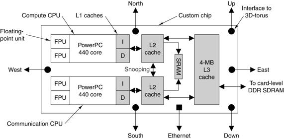
connection topology used in the BlueGene is a three–dimensional torus. Each processor chip is connected to six other
processor chips. The connections are
called “North”, “East”, “South”, “West”, “Up”, and “Down”.
The Custom Processor
Chip
IBM
intended the BlueGene line for general commercial and research
applications. Because of this, the
company elected to produce the processor chips from available commercial cores.
Each
processor chip has two PowerPC 440 cores operating at 700 MHz. The configuration of the chip, with its
multiple caches is shown in the figure below.
Note that only one of the two cores is dedicated to computation, the
other is dedicated to handling communications.
In a
recent upgrade (June 2007), IBM upgraded this chip to hold four PowerPC 450
cores operating at 850 MHz. In November
2007, the new computer, called the BlueGene/P achieved a sustained performance
of 167 teraflops. This design obviously
has some “growing room”.
The
BlueGene/L Hierarchy
The
65,536 BlueGene/L is designed in a hierarchical fashion. There are two chips per card,
16 cards per board, 32 boards per cabinet, and 64 cabinets in the system.
We shall
see that the MPP systems manufactured by Cray, Inc. follow the same design
philosophy.
It seems
that this organization will become common for large MPP systems.
The AMD
Opteron
Before
continuing with our discussion of MPP systems, let us stop and examine the chip
that has recently become the favorite for use as the processor, of which there
are thousands.
This
chip is the AMD Opteron, which is a 64–bit processor that can operate in three
modes.
In legacy mode, the Opteron runs standard
Pentium binary programs unmodified.
In compatibility mode, the operating
system runs in full 64–bit mode, but applications
must run in 32–bit mode.
In 64–bit mode, all programs can issue
64–bit addresses; both 32–bit and 64–bit
programs can run simultaneously in this mode.
The
Opteron has an integrated memory controller, which runs at the speed of the processor
clock.
This improves memory performance. It can
manage 32 GB of memory.
The
Opteron comes in single–core, dual–core, or quad–core processors. The standard clock rates for these processors
range from 1.7 to 2.3 GHz.
The Red
Storm by Cray, Inc.
The Red
Storm is a MPP system in operation at Sandia National Laboratory. This lab, operated by Lockheed Martin, doe
classified work for the U.S. Department of Energy. Much of this work supports the design of
nuclear weapons. The simulation of
nuclear weapon detonations, which is very computationally intensive, has
replaced actual testing as a way to verify designs.
In 2002,
Sandia selected Cray, Inc. to build a replacement for its current MPP, called
ASCI Red. This system had 1.2 terabytes
of RAM and operated at a peak rate of 3 teraflops.
The Red
Storm was delivered in August 2004 and upgraded in 2006 [Ref. 9]. The Red Storm now uses dual–core AMD Opterons,
operating at 2.4 GHz. Each Opteron has 4 GB of RAM and a dedicated custom
network processor called the Seastar,
manufactured by IBM.
Almost
all data traffic between processors moves through the Seastar network, so great
care was taken in its design. This is
the only chip that is custom–made for the project.
The next
step in the architecture hierarchy is the board,
which holds four complete Opteron systems (four CPU’s, 16 GB RAM, four Seastar
units), a 100 megabit per second Ethernet chip, and a RAS (Reliability,
Availability, and Service) processor to facilitate fault location.
The next
step in the hierarchy is the card cage,
which comprises eight boards inserted into a backplane. Three card cages and their supporting power
units are placed into a cabinet.
The full Red Storm system comprises 108 cabinets, for
a total of 10,836 Opterons and 10 terabytes of SDRAM. Its theoretical peak performance is 124
teraflops, with a sustained rate of 101 teraflops.
Security
Implications of the Architecture
In the
world on national laboratories there are special requirements on the
architecture of computers that might be used to process classified data. The Red Storm at Sandia routinely processes
data from which the detailed design of current
The
solution to the security problem was to partition Red Storm into classified and
unclassified sections. This partitioning
was done by mechanical switches, which would completely isolate one section
from another. There are three sections:
classified, unclassified, and a switchable section.
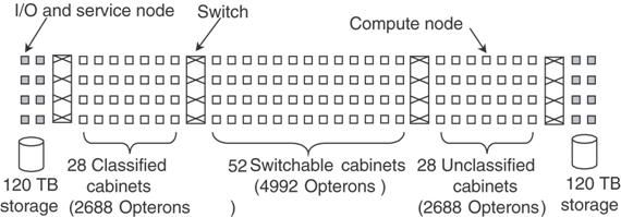
The
figure above, taken from Tanenbaum [Ref. 4], shows the configuration as it was
in 2005.
The Cray
XT5h
The Cray
XT3 is a commercial design based on the Red Storm installed at Sandia National
Labs.
The Cray
XT3 led to the development of the Cray XT4 and Cray XT5, the latest in the
line.
The XT5
follows the Red Storm approach in using a large number of AMD Opteron processors. The processor interconnect uses the same
three–dimensional torus as found in the IBM BlueGene and presumably in the Cray
Red Storm. The network processor has
been upgraded to a system called ‘Seastar 2+”; each switch having six 9.6
GB/second router–to–router ports.
The Cray
XT5h is a modified XT5, adding vector coprocessors and FPGA (Field Programmable
Gate Array) accelerators. FPGA
processors might be used to handle specific calculations, such as Fast Fourier
Transforms, which often run faster on these units than on general purpose
processors.
In April
2008, Cray, Inc. was chosen to deliver an XT4 to the
The Google
Cluster
We now
examine a loosely–coupled cluster design that is used at Google, the company providing
the popular search engine. We begin by
listing the goals and constraints of the design.
There
are two primary goals for the design.
1. To
provide key–word search of all the pages in the World Wide Web, returning
answers
in not more than 0.5 seconds
(a figure based on human tolerance for delays).
2. To
“crawl the web”, constantly examining pages on the World Wide Web and indexing
them for efficient
search. This process must be continuous
in order to keep the index current.
There
are two primary constraints on the design.
1. To
obtain the best performance for the price.
For this reason, high–end servers are eschewed
in favor of the cheaper
mass–market computers.
2. To
provide reliable service, allowing for components that will fail. Towards that end,
every component is replicated,
and maintenance is constant.
What
makes this design of interest to our class is the choice made in creating the
cluster. It could have been created from
a small number of Massively Parallel Processors or a larger number of closely
coupled high–end servers, but it was not.
It could have used a number of RAID servers, but it did not. The goal was to use commercial technology and
replicate everything.
According to our textbook [Ref. 1, page 9–39], the
company has not suffered a service outage
since it was a few months old, possibly in late 1998 or early 1999.
The Google
Process
We begin
by noting that the success of the cluster idea was due to the fact that the
processing of a query is one that can easily be partitioned into independent
cooperating processes.
Here is
a depiction of the Google process, taken from Tanenbaum [Ref. 4, page 629].
The Google
Process: Sequence of Actions
The
process of handling a web query always involves a number of cooperating
processors.
1. When the query arrives at the data center, it
is first handled by a load balancer. This load
balancer will select three other
computers, based on processing load, to handle the query.
2. The load balancer selects one each from the
available spell checkers, query handlers, and
advertisement servers. It sends the query to all three in parallel.
3. The spell checker will check for alternate
spellings and attempt to correct misspellings.
4. The advertisement server will select a number
of ads to be placed on the final display,
based on key words in the query.
5. The query handler will break the query into
“atomic units” and pass each unit to a
distinct index server. For example, a query for “Google corporate
history” would generate
three searches, each handled by a
distinct index server.
6. The query handler combines the results of the
“atomic queries” into one result. In the
example
above, a logical AND is performed;
the result must have been found in all three atomic queries.
7. Based on the document identifiers resulting
from the logical combination, the query handler
accesses the document servers and
retrieves links to the target web pages.
Google uses a proprietary algorithm for ranking
responses to queries. The average query
involves processing about 100 megabytes of data. Recall that this is to be done in under a
half of a second.
The Google
Cluster
The
typical Google cluster comprises 5120 PC’s, two 128–port Ethernet switches, 64
racks each with its own switch, and a number of other components. A depiction is shown below.
Note the redundancy built into the switches and the
two incoming lines from the Internet.
Blade
Servers and Blade Enclosures
Blade enclosures represent a refinement of the rack mounts for computers, as found in
the Google cluster. In a blade
enclosure, each blade server is a
standard design computer with many components removed for space and power
considerations.
The
common functions (such as power, cooling, networking, and processor
interconnect) are provided by the blade enclosure, so that the blade server is a
very efficient design.
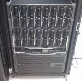 The figure at left shows an HP Proliant blade
enclosure with what appears to be sixteen blade servers, arranged in two racks
of 8.
The figure at left shows an HP Proliant blade
enclosure with what appears to be sixteen blade servers, arranged in two racks
of 8.
Typically
blade servers are “hot swappable”, meaning that a unit can be removed without
shutting down and rebooting all of the servers in the enclosure. This greatly facilitates maintenance.
Essentially
a blade enclosure is a closely coupled multicomputer. Typical uses include web hosting, database
servers, e–mail servers, and other forms of cluster computing.
According
to Wikipedia [Ref. 10], the first unit called a “blade server” was developed by
RTX Technologies of Houston, TX and shipped in May 2001.
It is interesting to speculate about the Google
design, had blade servers been available in the late 1990’s when Google was
starting up.
Radio SETI
This
information is taken from the SETI@Home web page [Ref. 7].
SETI is the acronym for “Search for Extra–Terrestrial Intelligence”. Radio SETI refers to the use of radio
receivers to detect signals that might indicate another intelligent species in
the universe.
The SETI
antennas regularly detect signals from a species that is reputed to be
intelligent; unfortunately that is us on this planet. A great deal of computation is required to
filter the noise and human–generated signals from the signals detected,
possibly leaving signals from sources that might be truly extraterrestrial.
Part of
this processing is to remove extraterrestrial signals that, while very
interesting, are due to natural sources.
Such are the astronomical objects originally named “Little Green Men”,
but later named as “quasars” and now fully explained by modern astrophysical
theory.
Radio
SETI was started under a modest grant and involved the use of dedicated radio
antennas and supercomputers (the Cray–1 ?) located on the site.
In 1995,
David Gedye proposed a cheaper data–processing solution: create a virtual
supercomputer composed of large numbers of computers connected by the global
Internet. SETI@home was launched in May
1999 and continues active to this day [May 2008].
Many
computer companies, such as Sun Microsystems, routinely run the SETI@home on
their larger systems for about 24 hours as a way of testing before shipping to
the customer.
A Radio
Telescope
Here is
a picture of the very large radio telescope at Arecibo in Puerto Rico.
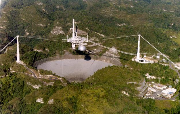
This is the source of data to be processed by the
SETI@home project at Berkeley. Arecibo
produces about 35 gigabytes of data per day.
These data are given a cursory examination and sent by U.S. Mail to the
Berkeley campus in California; Arecibo lacks a high–speed Internet connection.
The Radio
SETI Process
Radio
SETI monitors a 2.5 MHz radio band from 1418.75 to 1421.25 MHz. This band, centered at the 1420 MHz frequency
called the “Hydrogen line” is thought to be optimal for interstellar
transmissions. The data are recorded in
analog mode and digitized later.
When the
analog data arrive at Berkeley, they are broken into 250 kilobyte chunks,
called “work units” by a software program called “Splitter” Each work unit represents a 9,766 Hz slice of
the 2,500 kHz spectrum. This analog
signal is digitized at 20,000 samples per second.
Participants
in the Radio SETI project are sent these work units, each representing about
107 seconds of analog data. The entire
packet, along with the work unit, is about 340 kilobytes.
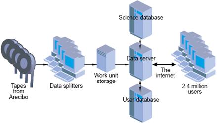
This figure shows the processing network, including
the four servers at Berkeley and the 2.4 million personal computers that form
the volunteer network.
References
In this lecture, material from one or more of the
following references has been used.
1. Computer
Organization and Design, David A. Patterson & John L. Hennessy,
Morgan Kaufmann, (3rd
Edition, Revised Printing) 2007, (The course textbook)
ISBN 978 – 0 – 12 – 370606 – 5.
2. Computer
Architecture: A Quantitative Approach, John L. Hennessy and
David A. Patterson, Morgan
Kauffman, 1990. There is a later
edition.
ISBN 1 – 55860 – 069 – 8.
3. High–Performance
Computer Architecture, Harold S. Stone,
Addison–Wesley (Third Edition),
1993. ISBN 0 – 201 – 52688 – 3.
4. Structured
Computer Organization, Andrew S. Tanenbaum,
Pearson/Prentice–Hall (Fifth
Edition), 2006. ISBN 0 – 13 – 148521 – 0
5. Computer Architecture,
Robert J. Baron and Lee Higbie,
Addison–Wesley Publishing Company,
1992, ISBN 0 – 201 – 50923 – 7.
6. W. A. Wulf and S. P. Harbison, “Reflections in a pool of
processors / An
experience report on C.mmp/Hydra”,
Proceedings of the National Computer
Conference (AFIPS), June 1978.
Web Links
7. The
link describing SETI at home: http://setiathome.berkeley.edu/
8. The
web site for Cray, Inc.: http://www.cray.com/
9. The
link for Red Storm at Sandia National Labs: http://www.sandia.gov/ASC/redstorm.html
10. The
Wikipedia article on blade servers: http://en.wikipedia.org/wiki/Blade_server